Bezier Curve-
Bezier Curve may be defined as-
- Bezier Curve is parametric curve defined by a set of control points.
- Two points are ends of the curve.
- Other points determine the shape of the curve.
The concept of bezier curves was given by Pierre Bezier.
Bezier Curve Example-
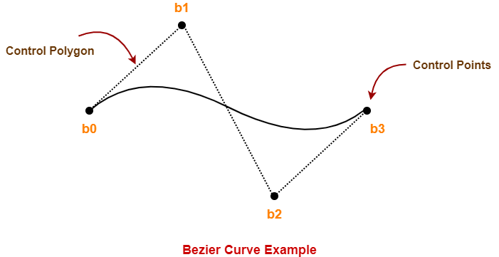
The following curve is an example of a bezier curve-
Here,
- This bezier curve is defined by a set of control points b0, b1, b2 and b3.
- Points b0 and b3 are ends of the curve.
- Points b1 and b2 determine the shape of the curve.
Bezier Curve Properties-
Few important properties of a bezier curve are-
Property-01:
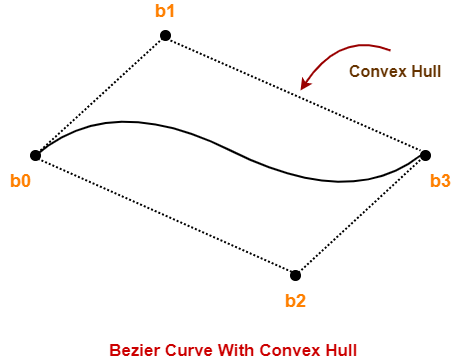
Bezier curve is always contained within a polygon called as convex hull of its control points.
Property-02:
- Bezier curve generally follows the shape of its defining polygon.
- The first and last points of the curve are coincident with the first and last points of the defining polygon.
Property-03:
The degree of the polynomial defining the curve segment is one less than the total number of control points.
Degree = Number of Control Points – 1
Property-04:
The order of the polynomial defining the curve segment is equal to the total number of control points.
Order = Number of Control Points
Property-05:
- Bezier curve exhibits the variation diminishing property.
- It means the curve do not oscillate about any straight line more often than the defining polygon.
Bezier Curve Equation-
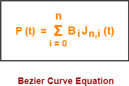
A bezier curve is parametrically represented by-
Here,
- t is any parameter where 0 <= t <= 1
- P(t) = Any point lying on the bezier curve
- Bi = ith control point of the bezier curve
- n = degree of the curve
- Jn,i(t) = Blending function = C(n,i)ti(1-t)n-i where C(n,i) = n! / i!(n-i)!
Cubic Bezier Curve-
- Cubic bezier curve is a bezier curve with degree 3.
- The total number of control points in a cubic bezier curve is 4.
Example-
The following curve is an example of a cubic bezier curve-

Here,
- This curve is defined by 4 control points b0, b1, b2 and b3.
- The degree of this curve is 3.
- So, it is a cubic bezier curve.
Cubic Bezier Curve Equation-
The parametric equation of a bezier curve is-

Substituting n = 3 for a cubic bezier curve, we get-

Expanding the above equation, we get-
P (t) = B0J3,0(t) + B1J3,1(t) + B2J3,2(t) + B3J3,3(t) ………..(1)
Now,
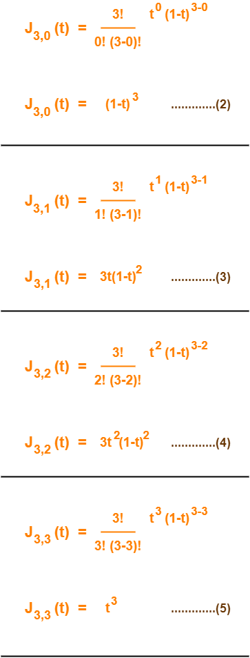
Using (2), (3), (4) and (5) in (1), we get-
P(t) = B0(1-t)3 + B13t(1-t)2 + B23t2(1-t) + B3t3
This is the required parametric equation for a cubic bezier curve.
Applications of Bezier Curves-
Bezier curves have their applications in the following fields-
1. Computer Graphics-
- Bezier curves are widely used in computer graphics to model smooth curves.
- The curve is completely contained in the convex hull of its control points.
- So, the points can be graphically displayed & used to manipulate the curve intuitively.
2. Animation-
- Bezier curves are used to outline movement in animation applications such as Adobe Flash and synfig.
- Users outline the wanted path in bezier curves.
- The application creates the needed frames for the object to move along the path.
- For 3D animation, bezier curves are often used to define 3D paths as well as 2D curves.
3. Fonts-
- True type fonts use composite bezier curves composed of quadratic bezier curves.
- Modern imaging systems like postscript, asymptote etc use composite bezier curves composed of cubic bezier curves for drawing curved shapes.
PRACTICE PROBLEMS BASED ON BEZIER CURVE IN COMPUTER GRAPHICS-
Problem-01:
Given a bezier curve with 4 control points-
B0[1 0] , B1[3 3] , B2[6 3] , B3[8 1]
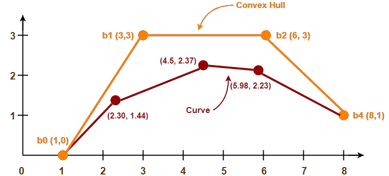
Determine any 5 points lying on the curve. Also, draw a rough sketch of the curve.
Solution-
We have-
- The given curve is defined by 4 control points.
- So, the given curve is a cubic bezier curve.
The parametric equation for a cubic bezier curve is-
P(t) = B0(1-t)3 + B13t(1-t)2 + B23t2(1-t) + B3t3
Substituting the control points B0, B1, B2 and B3, we get-
P(t) = [1 0](1-t)3 + [3 3]3t(1-t)2 + [6 3]3t2(1-t) + [8 1]t3 ……..(1)
Now,
To get 5 points lying on the curve, assume any 5 values of t lying in the range 0 <= t <= 1.
Let 5 values of t are 0, 0.2, 0.5, 0.7, 1
For t = 0:
Substituting t=0 in (1), we get-
P(0) = [1 0](1-0)3 + [3 3]3(0)(1-t)2 + [6 3]3(0)2(1-0) + [8 1](0)3
P(0) = [1 0] + 0 + 0 + 0
P(0) = [1 0]
For t = 0.2:
Substituting t=0.2 in (1), we get-
P(0.2) = [1 0](1-0.2)3 + [3 3]3(0.2)(1-0.2)2 + [6 3]3(0.2)2(1-0.2) + [8 1](0.2)3
P(0.2) = [1 0](0.8)3 + [3 3]3(0.2)(0.8)2 + [6 3]3(0.2)2(0.8) + [8 1](0.2)3
P(0.2) = [1 0] x 0.512 + [3 3] x 3 x 0.2 x 0.64 + [6 3] x 3 x 0.04 x 0.8 + [8 1] x 0.008
P(0.2) = [1 0] x 0.512 + [3 3] x 0.384 + [6 3] x 0.096 + [8 1] x 0.008
P(0.2) = [0.512 0] + [1.152 1.152] + [0.576 0.288] + [0.064 0.008]
P(0.2) = [2.304 1.448]
For t = 0.5:
Substituting t=0.5 in (1), we get-
P(0.5) = [1 0](1-0.5)3 + [3 3]3(0.5)(1-0.5)2 + [6 3]3(0.5)2(1-0.5) + [8 1](0.5)3
P(0.5) = [1 0](0.5)3 + [3 3]3(0.5)(0.5)2 + [6 3]3(0.5)2(0.5) + [8 1](0.5)3
P(0.5) = [1 0] x 0.125 + [3 3] x 3 x 0.5 x 0.25 + [6 3] x 3 x 0.25 x 0.5 + [8 1] x 0.125
P(0.5) = [1 0] x 0.125 + [3 3] x 0.375 + [6 3] x 0.375 + [8 1] x 0.125
P(0.5) = [0.125 0] + [1.125 1.125] + [2.25 1.125] + [1 0.125]
P(0.5) = [4.5 2.375]
For t = 0.7:
Substituting t=0.7 in (1), we get-
P(t) = [1 0](1-t)3 + [3 3]3t(1-t)2 + [6 3]3t2(1-t) + [8 1]t3
P(0.7) = [1 0](1-0.7)3 + [3 3]3(0.7)(1-0.7)2 + [6 3]3(0.7)2(1-0.7) + [8 1](0.7)3
P(0.7) = [1 0](0.3)3 + [3 3]3(0.7)(0.3)2 + [6 3]3(0.7)2(0.3) + [8 1](0.7)3
P(0.7) = [1 0] x 0.027 + [3 3] x 3 x 0.7 x 0.09 + [6 3] x 3 x 0.49 x 0.3 + [8 1] x 0.343
P(0.7) = [1 0] x 0.027 + [3 3] x 0.189 + [6 3] x 0.441 + [8 1] x 0.343
P(0.7) = [0.027 0] + [0.567 0.567] + [2.646 1.323] + [2.744 0.343]
P(0.7) = [5.984 2.233]
For t = 1:
Substituting t=1 in (1), we get-
P(1) = [1 0](1-1)3 + [3 3]3(1)(1-1)2 + [6 3]3(1)2(1-1) + [8 1](1)3
P(1) = [1 0] x 0 + [3 3] x 3 x 1 x 0 + [6 3] x 3 x 1 x 0 + [8 1] x 1
P(1) = 0 + 0 + 0 + [8 1]
P(1) = [8 1]
Following is the required rough sketch of the curve-
To gain better understanding about Bezier Curves in Computer Graphics,
Get more notes and other study material of Computer Graphics.
Watch video lectures by visiting our YouTube channel LearnVidFun.