Travelling Salesman Problem-

 

You are given-

• A set of some cities
• Distance between every pair of cities

 

Travelling Salesman Problem states-

• A salesman has to visit every city exactly once.
• He has to come back to the city from where he starts his journey.
• What is the shortest possible route that the salesman must follow to complete his tour?

 

Example-

 

The following graph shows a set of cities and distance between every pair of cities-

 

 

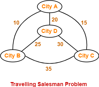
If salesman starting city is A, then a TSP tour in the graph is-

A → B → D → C → A

 

Cost of the tour

= 10 + 25 + 30 + 15

= 80 units

 

In this article, we will discuss how to solve travelling salesman problem using branch and bound approach with example.

 

PRACTICE PROBLEM BASED ON TRAVELLING SALESMAN PROBLEM USING BRANCH AND BOUND APPROACH-

 

Problem-

 

Solve Travelling Salesman Problem using Branch and Bound Algorithm in the following graph-

 

 

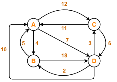
Solution-

 

Step-01:

 

Write the initial cost matrix and reduce it-

 

 

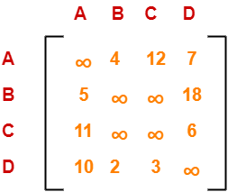
Rules To reduce a matrix, perform the row reduction and column reduction of the matrix separately. A row or a column is said to be reduced if it contains at least one entry ‘0’ in it.

 

Row Reduction-

 

Consider the rows of above matrix one by one.

 

If the row already contains an entry ‘0’, then-

• There is no need to reduce that row.

 

If the row does not contains an entry ‘0’, then-

• Reduce that particular row.
• Select the least value element from that row.
• Subtract that element from each element of that row.
• This will create an entry ‘0’ in that row, thus reducing that row.

 

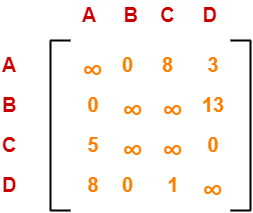
Following this, we have-

• Reduce the elements of row-1 by 4.
• Reduce the elements of row-2 by 5.
• Reduce the elements of row-3 by 6.
• Reduce the elements of row-4 by 2.

 

Performing this, we obtain the following row-reduced matrix-

 

 

Column Reduction-

 

Consider the columns of above row-reduced matrix one by one.

 

If the column already contains an entry ‘0’, then-

• There is no need to reduce that column.

 

If the column does not contains an entry ‘0’, then-

• Reduce that particular column.
• Select the least value element from that column.
• Subtract that element from each element of that column.
• This will create an entry ‘0’ in that column, thus reducing that column.

 

Following this, we have-

• There is no need to reduce column-1.
• There is no need to reduce column-2.
• Reduce the elements of column-3 by 1.
• There is no need to reduce column-4.

 

Performing this, we obtain the following column-reduced matrix-

 

 

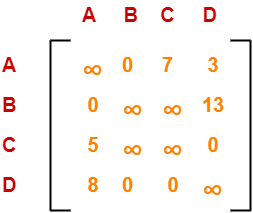
Finally, the initial distance matrix is completely reduced.

Now, we calculate the cost of node-1 by adding all the reduction elements.

 

Cost(1)

= Sum of all reduction elements

= 4 + 5 + 6 + 2 + 1

= 18

 

Step-02:

 

• We consider all other vertices one by one.
• We select the best vertex where we can land upon to minimize the tour cost.

 

Choosing To Go To Vertex-B: Node-2 (Path A → B)

 

• From the reduced matrix of step-01, M[A,B] = 0
• Set row-A and column-B to ∞
• Set M[B,A] = ∞

 

Now, resulting cost matrix is-

 

 

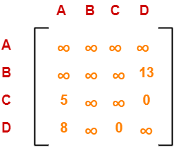
Now,

• We reduce this matrix.
• Then, we find out the cost of node-02.

 

Row Reduction-

 

• We can not reduce row-1 as all its elements are ∞.
• Reduce all the elements of row-2 by 13.
• There is no need to reduce row-3.
• There is no need to reduce row-4.

 

Performing this, we obtain the following row-reduced matrix-

 

 

Column Reduction-

 

• Reduce the elements of column-1 by 5.
• We can not reduce column-2 as all its elements are ∞.
• There is no need to reduce column-3.
• There is no need to reduce column-4.

 

Performing this, we obtain the following column-reduced matrix-

 

 

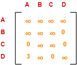
Finally, the matrix is completely reduced.

Now, we calculate the cost of node-2.

 

Cost(2)

= Cost(1) + Sum of reduction elements + M[A,B]

= 18 + (13 + 5) + 0

= 36

 

Choosing To Go To Vertex-C: Node-3 (Path A → C)

 

• From the reduced matrix of step-01, M[A,C] = 7
• Set row-A and column-C to ∞
• Set M[C,A] = ∞

 

Now, resulting cost matrix is-

 

 

Now,

• We reduce this matrix.
• Then, we find out the cost of node-03.

 

Row Reduction-

 

• We can not reduce row-1 as all its elements are ∞.
• There is no need to reduce row-2.
• There is no need to reduce row-3.
• There is no need to reduce row-4.

 

Thus, the matrix is already row-reduced.

 

Column Reduction-

 

• There is no need to reduce column-1.
• There is no need to reduce column-2.
• We can not reduce column-3 as all its elements are ∞.
• There is no need to reduce column-4.

 

Thus, the matrix is already column reduced.

Finally, the matrix is completely reduced.

Now, we calculate the cost of node-3.

 

Cost(3)

= Cost(1) + Sum of reduction elements + M[A,C]

= 18 + 0 + 7

= 25

 

Choosing To Go To Vertex-D: Node-4 (Path A → D)

 

• From the reduced matrix of step-01, M[A,D] = 3
• Set row-A and column-D to ∞
• Set M[D,A] = ∞

 

Now, resulting cost matrix is-

 

 

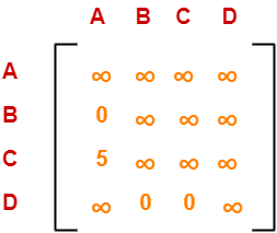
Now,

• We reduce this matrix.
• Then, we find out the cost of node-04.

 

Row Reduction-

 

• We can not reduce row-1 as all its elements are ∞.
• There is no need to reduce row-2.
• Reduce all the elements of row-3 by 5.
• There is no need to reduce row-4.

 

Performing this, we obtain the following row-reduced matrix-

 

 

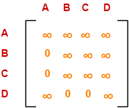
Column Reduction-

 

• There is no need to reduce column-1.
• There is no need to reduce column-2.
• There is no need to reduce column-3.
• We can not reduce column-4 as all its elements are ∞.

 

Thus, the matrix is already column-reduced.

Finally, the matrix is completely reduced.

Now, we calculate the cost of node-4.

 

Cost(4)

= Cost(1) + Sum of reduction elements + M[A,D]

= 18 + 5 + 3

= 26

 

Thus, we have-

• Cost(2) = 36 (for Path A → B)
• Cost(3) = 25 (for Path A → C)
• Cost(4) = 26 (for Path A → D)

 

We choose the node with the lowest cost.

Since cost for node-3 is lowest, so we prefer to visit node-3.

Thus, we choose node-3 i.e. path A → C.

 

Step-03:

 

We explore the vertices B and D from node-3.

We now start from the cost matrix at node-3 which is-

 

 

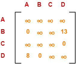
Cost(3) = 25

 

Choosing To Go To Vertex-B: Node-5 (Path A → C → B)

 

• From the reduced matrix of step-02, M[C,B] = ∞
• Set row-C and column-B to ∞
• Set M[B,A] = ∞

 

Now, resulting cost matrix is-

 

 

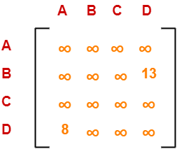
Now,

• We reduce this matrix.
• Then, we find out the cost of node-5.

 

Row Reduction-

 

• We can not reduce row-1 as all its elements are ∞.
• Reduce all the elements of row-2 by 13.
• We can not reduce row-3 as all its elements are ∞.
• Reduce all the elements of row-4 by 8.

 

Performing this, we obtain the following row-reduced matrix-

 

 

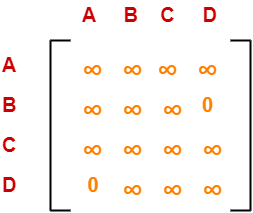
Column Reduction-

 

• There is no need to reduce column-1.
• We can not reduce column-2 as all its elements are ∞.
• We can not reduce column-3 as all its elements are ∞.
• There is no need to reduce column-4.

 

Thus, the matrix is already column reduced.

Finally, the matrix is completely reduced.

Now, we calculate the cost of node-5.

 

Cost(5)

= cost(3) + Sum of reduction elements + M[C,B]

= 25 + (13 + 8) + ∞

= ∞

 

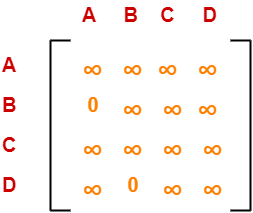
Choosing To Go To Vertex-D: Node-6 (Path A → C → D)

 

• From the reduced matrix of step-02, M[C,D] = ∞
• Set row-C and column-D to ∞
• Set M[D,A] = ∞

 

Now, resulting cost matrix is-

 

 

Now,

• We reduce this matrix.
• Then, we find out the cost of node-6.

 

Row Reduction-

 

• We can not reduce row-1 as all its elements are ∞.
• There is no need to reduce row-2.
• We can not reduce row-3 as all its elements are ∞.
• We can not reduce row-4 as all its elements are ∞.

 

Thus, the matrix is already row reduced.

 

Column Reduction-

 

• There is no need to reduce column-1.
• We can not reduce column-2 as all its elements are ∞.
• We can not reduce column-3 as all its elements are ∞.
• We can not reduce column-4 as all its elements are ∞.

 

Thus, the matrix is already column reduced.

Finally, the matrix is completely reduced.

Now, we calculate the cost of node-6.

 

Cost(6)

= cost(3) + Sum of reduction elements + M[C,D]

= 25 + 0 + 0

= 25

 

Thus, we have-

• Cost(5) = ∞ (for Path A → C → B)
• Cost(6) = 25 (for Path A → C → D)

 

We choose the node with the lowest cost.

Since cost for node-6 is lowest, so we prefer to visit node-6.

Thus, we choose node-6 i.e. path C → D.

 

Step-04:

 

We explore vertex B from node-6.

We start with the cost matrix at node-6 which is-

 

 

Cost(6) = 25

 

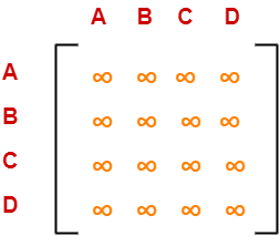
Choosing To Go To Vertex-B: Node-7 (Path A → C → D → B)

 

• From the reduced matrix of step-03, M[D,B] = 0
• Set row-D and column-B to ∞
• Set M[B,A] = ∞

 

Now, resulting cost matrix is-

 

 

Now,

• We reduce this matrix.
• Then, we find out the cost of node-7.

 

Row Reduction-

 

• We can not reduce row-1 as all its elements are ∞.
• We can not reduce row-2 as all its elements are ∞.
• We can not reduce row-3 as all its elements are ∞.
• We can not reduce row-4 as all its elements are ∞.

 

Column Reduction-

 

• We can not reduce column-1 as all its elements are ∞.
• We can not reduce column-2 as all its elements are ∞.
• We can not reduce column-3 as all its elements are ∞.
• We can not reduce column-4 as all its elements are ∞.

 

Thus, the matrix is already column reduced.

Finally, the matrix is completely reduced.

All the entries have become ∞.

Now, we calculate the cost of node-7.

 

Cost(7)

= cost(6) + Sum of reduction elements + M[D,B]

= 25 + 0 + 0

= 25

 

Thus,

• Optimal path is: A → C → D → B → A
• Cost of Optimal path = 25 units

 

To gain better understanding about Travelling Salesman Problem,

Watch this Video Lecture

 

Get more notes and other study material of Design and Analysis of Algorithms.

Watch video lectures by visiting our YouTube channel LearnVidFun.