Tag: Data Structures and Algorithms

Binary Search Tree Insertion | BST Deletion

Binary Search Tree-


Before you go through this article, make sure that you have gone through the previous article on Binary Search Trees.


Binary search tree (BST) is a special kind of binary tree where each node contains-

  • Only larger values in its right subtree.
  • Only smaller values in its left subtree.


In this article, we will discuss about Binary Search Tree Operations.


Binary Search Tree Operations-


Commonly performed operations on binary search tree are-


  1. Search Operation
  2. Insertion Operation
  3. Deletion Operation


1. Search Operation-


Search Operation is performed to search a particular element in the Binary Search Tree.


Rules-


For searching a given key in the BST,

  • Compare the key with the value of root node.
  • If the key is present at the root node, then return the root node.
  • If the key is greater than the root node value, then recur for the root node’s right subtree.
  • If the key is smaller than the root node value, then recur for the root node’s left subtree.


Example-


Consider key = 45 has to be searched in the given BST-
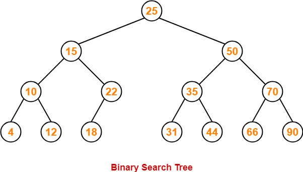


  • We start our search from the root node 25.
  • As 45 > 25, so we search in 25’s right subtree.
  • As 45 < 50, so we search in 50’s left subtree.
  • As 45 > 35, so we search in 35’s right subtree.
  • As 45 > 44, so we search in 44’s right subtree but 44 has no subtrees.
  • So, we conclude that 45 is not present in the above BST.


2. Insertion Operation-


Insertion Operation is performed to insert an element in the Binary Search Tree.


Rules-


The insertion of a new key always takes place as the child of some leaf node.

For finding out the suitable leaf node,

  • Search the key to be inserted from the root node till some leaf node is reached.
  • Once a leaf node is reached, insert the key as child of that leaf node.


Example-


Consider the following example where key = 40 is inserted in the given BST-
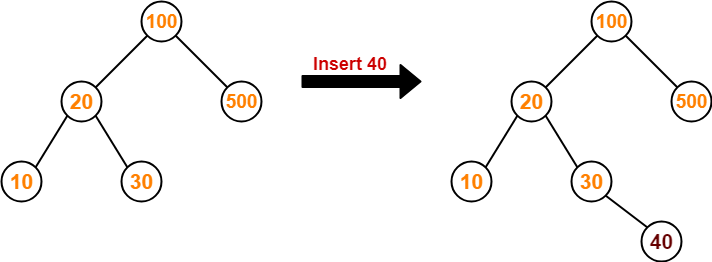


  • We start searching for value 40 from the root node 100.
  • As 40 < 100, so we search in 100’s left subtree.
  • As 40 > 20, so we search in 20’s right subtree.
  • As 40 > 30, so we add 40 to 30’s right subtree.


3. Deletion Operation-


Deletion Operation is performed to delete a particular element from the Binary Search Tree.


When it comes to deleting a node from the binary search tree, following three cases are possible-


Case-01: Deletion Of A Node Having No Child (Leaf Node)-


Just remove / disconnect the leaf node that is to deleted from the tree.


Example-


Consider the following example where node with value = 20 is deleted from the BST-


Case-02: Deletion Of A Node Having Only One Child-


Just make the child of the deleting node, the child of its grandparent.


Example-


Consider the following example where node with value = 30 is deleted from the BST-


Case-02: Deletion Of A Node Having Two Children-


A node with two children may be deleted from the BST in the following two ways-


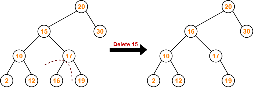
Method-01:


  • Visit to the right subtree of the deleting node.
  • Pluck the least value element called as inorder successor.
  • Replace the deleting element with its inorder successor.


Example-


Consider the following example where node with value = 15 is deleted from the BST-


Method-02:


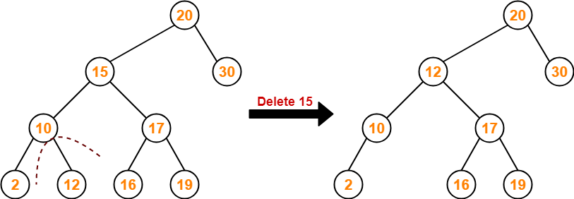
  • Visit to the left subtree of the deleting node.
  • Pluck the greatest value element called as inorder predecessor.
  • Replace the deleting element with its inorder predecessor.


Example-


Consider the following example where node with value = 15 is deleted from the BST-


To gain better understanding about BST Operations,

Watch this Video Lecture


Download Handwritten Notes Here-


Next Article- Time Complexity of BST Operations


Get more notes and other study material of Data Structures.

Watch video lectures by visiting our YouTube channel LearnVidFun.

Dijkstra Algorithm | Example | Time Complexity

Dijkstra Algorithm-


  • Dijkstra Algorithm is a very famous greedy algorithm.
  • It is used for solving the single source shortest path problem.
  • It computes the shortest path from one particular source node to all other remaining nodes of the graph.


Also Read- Shortest Path Problem


Conditions-


It is important to note the following points regarding Dijkstra Algorithm-

  • Dijkstra algorithm works only for connected graphs.
  • Dijkstra algorithm works only for those graphs that do not contain any negative weight edge.
  • The actual Dijkstra algorithm does not output the shortest paths.
  • It only provides the value or cost of the shortest paths.
  • By making minor modifications in the actual algorithm, the shortest paths can be easily obtained.
  • Dijkstra algorithm works for directed as well as undirected graphs.


Dijkstra Algorithm-


dist[S] ← 0                                                  // The distance to source vertex is set to 0

Π[S] ← NIL                                                   // The predecessor of source vertex is set as NIL

for all v ∈ V - {S}                                          // For all other vertices

        do dist[v] ← ∞                                       // All other distances are set to ∞

        Π[v] ← NIL                                           // The predecessor of all other vertices is set as NIL

S ← ∅                                                        // The set of vertices that have been visited 'S' is initially empty

Q ← V                                                        // The queue 'Q' initially contains all the vertices

while Q ≠ ∅                                                  // While loop executes till the queue is not empty

        do u ← mindistance (Q, dist)                         // A vertex from Q with the least distance is selected

        S ← S ∪ {u}                                          // Vertex 'u' is added to 'S' list of vertices that have been visited

for all v ∈ neighbors[u]                                     // For all the neighboring vertices of vertex 'u'

        do if dist[v] > dist[u] + w(u,v)                     // if any new shortest path is discovered

                then dist[v] ← dist[u] + w(u,v)              // The new value of the shortest path is selected

return dist


Implementation-


The implementation of above Dijkstra Algorithm is explained in the following steps-


Step-01:


In the first step. two sets are defined-

  • One set contains all those vertices which have been included in the shortest path tree.
  • In the beginning, this set is empty.
  • Other set contains all those vertices which are still left to be included in the shortest path tree.
  • In the beginning, this set contains all the vertices of the given graph.


Step-02:


For each vertex of the given graph, two variables are defined as-

  • Π[v] which denotes the predecessor of vertex ‘v’
  • d[v] which denotes the shortest path estimate of vertex ‘v’ from the source vertex.


Initially, the value of these variables is set as-

  • The value of variable ‘Π’ for each vertex is set to NIL i.e. Π[v] = NIL
  • The value of variable ‘d’ for source vertex is set to 0 i.e. d[S] = 0
  • The value of variable ‘d’ for remaining vertices is set to ∞ i.e. d[v] = ∞


Step-03:


The following procedure is repeated until all the vertices of the graph are processed-

  • Among unprocessed  vertices, a vertex with minimum value of variable ‘d’ is chosen.
  • Its outgoing edges are relaxed.
  • After relaxing the edges for that vertex, the sets created in step-01 are updated.


What is Edge Relaxation?


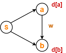
Consider the edge (a,b) in the following graph-


Here, d[a] and d[b] denotes the shortest path estimate for vertices a and b respectively from the source vertex ‘S’.

Now,

If d[a] + w < d[b]

then d[b] = d[a] + w and Π[b] = a

This is called as edge relaxation.


Time Complexity Analysis-


Case-01:


This case is valid when-

  • The given graph G is represented as an adjacency matrix.
  • Priority queue Q is represented as an unordered list.


Here,

  • A[i,j] stores the information about edge (i,j).
  • Time taken for selecting i with the smallest dist is O(V).
  • For each neighbor of i, time taken for updating dist[j] is O(1) and there will be maximum V neighbors.
  • Time taken for each iteration of the loop is O(V) and one vertex is deleted from Q.
  • Thus, total time complexity becomes O(V2).


Case-02:


This case is valid when-

  • The given graph G is represented as an adjacency list.
  • Priority queue Q is represented as a binary heap.


Here,

  • With adjacency list representation, all vertices of the graph can be traversed using BFS in O(V+E) time.
  • In min heap, operations like extract-min and decrease-key value takes O(logV) time.
  • So, overall time complexity becomes O(E+V) x O(logV) which is O((E + V) x logV) = O(ElogV)
  • This time complexity can be reduced to O(E+VlogV) using Fibonacci heap.


PRACTICE PROBLEM BASED ON DIJKSTRA ALGORITHM-


Problem-


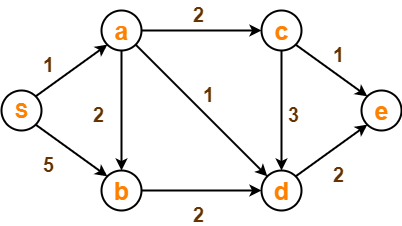
Using Dijkstra’s Algorithm, find the shortest distance from source vertex ‘S’ to remaining vertices in the following graph-


Also, write the order in which the vertices are visited.


Solution-


Step-01:


The following two sets are created-

  • Unvisited set : {S , a , b , c , d , e}
  • Visited set     : { }


Step-02:


The two variables  Π and d are created for each vertex and initialized as-

  • Π[S] = Π[a] = Π[b] = Π[c] = Π[d] = Π[e] = NIL
  • d[S] = 0
  • d[a] = d[b] = d[c] = d[d] = d[e] = ∞


Step-03:


  • Vertex ‘S’ is chosen.
  • This is because shortest path estimate for vertex ‘S’ is least.
  • The outgoing edges of vertex ‘S’ are relaxed.


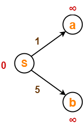
Before Edge Relaxation-


Now,

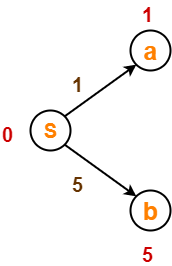
  • d[S] + 1 = 0 + 1 = 1 < ∞

∴ d[a] = 1 and Π[a] = S

  • d[S] + 5 = 0 + 5 = 5 < ∞

∴ d[b] = 5 and Π[b] = S


After edge relaxation, our shortest path tree is-


Now, the sets are updated as-

  • Unvisited set : {a , b , c , d , e}
  • Visited set : {S}


Step-04:


  • Vertex ‘a’ is chosen.
  • This is because shortest path estimate for vertex ‘a’ is least.
  • The outgoing edges of vertex ‘a’ are relaxed.


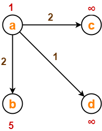
Before Edge Relaxation-


Now,

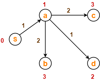
  • d[a] + 2 = 1 + 2 = 3 < ∞

∴ d[c] = 3 and Π[c] = a

  • d[a] + 1 = 1 + 1 = 2 < ∞

∴ d[d] = 2 and Π[d] = a

  • d[b] + 2 = 1 + 2 = 3 < 5

∴ d[b] = 3 and Π[b] = a


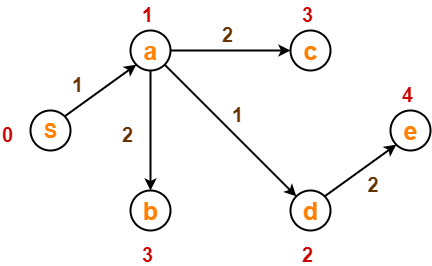
After edge relaxation, our shortest path tree is-


Now, the sets are updated as-

  • Unvisited set : {b , c , d , e}
  • Visited set : {S , a}


Step-05:


  • Vertex ‘d’ is chosen.
  • This is because shortest path estimate for vertex ‘d’ is least.
  • The outgoing edges of vertex ‘d’ are relaxed.


Before Edge Relaxation-


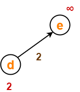
Now,

  • d[d] + 2 = 2 + 2 = 4 < ∞

∴ d[e] = 4 and Π[e] = d


After edge relaxation, our shortest path tree is-


Now, the sets are updated as-

  • Unvisited set : {b , c , e}
  • Visited set : {S , a , d}


Step-06:


  • Vertex ‘b’ is chosen.
  • This is because shortest path estimate for vertex ‘b’ is least.
  • Vertex ‘c’ may also be chosen since for both the vertices, shortest path estimate is least.
  • The outgoing edges of vertex ‘b’ are relaxed.


Before Edge Relaxation-


Now,

  • d[b] + 2 = 3 + 2 = 5 > 2

∴ No change


After edge relaxation, our shortest path tree remains the same as in Step-05.

Now, the sets are updated as-

  • Unvisited set : {c , e}
  • Visited set     : {S , a , d , b}


Step-07:


  • Vertex ‘c’ is chosen.
  • This is because shortest path estimate for vertex ‘c’ is least.
  • The outgoing edges of vertex ‘c’ are relaxed.


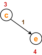
Before Edge Relaxation-


Now,

  • d[c] + 1 = 3 + 1 = 4 = 4

∴ No change


After edge relaxation, our shortest path tree remains the same as in Step-05.

Now, the sets are updated as-

  • Unvisited set : {e}
  • Visited set : {S , a , d , b , c}


Step-08:


  • Vertex ‘e’ is chosen.
  • This is because shortest path estimate for vertex ‘e’ is least.
  • The outgoing edges of vertex ‘e’ are relaxed.
  • There are no outgoing edges for vertex ‘e’.
  • So, our shortest path tree remains the same as in Step-05.


Now, the sets are updated as-

  • Unvisited set : { }
  • Visited set : {S , a , d , b , c , e}


Now,

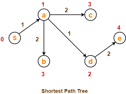
  • All vertices of the graph are processed.
  • Our final shortest path tree is as shown below.
  • It represents the shortest path from source vertex ‘S’ to all other remaining vertices.


The order in which all the vertices are processed is :

S , a , d , b , c , e.


To gain better understanding about Dijkstra Algorithm,

Watch this Video Lecture


Next Article- Floyd-Warshall Algorithm


Get more notes and other study material of Design and Analysis of Algorithms.

Watch video lectures by visiting our YouTube channel LearnVidFun.
0/1 Knapsack Problem | Dynamic Programming | Example

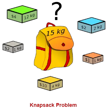
Knapsack Problem-


You are given the following-

  • A knapsack (kind of shoulder bag) with limited weight capacity.
  • Few items each having some weight and value.


The problem states-

Which items should be placed into the knapsack such that-

  • The value or profit obtained by putting the items into the knapsack is maximum.
  • And the weight limit of the knapsack does not exceed.


Knapsack Problem Variants-


Knapsack problem has the following two variants-

  1. Fractional Knapsack Problem
  2. 0/1 Knapsack Problem


In this article, we will discuss about 0/1 Knapsack Problem.


0/1 Knapsack Problem-


In 0/1 Knapsack Problem,

  • As the name suggests, items are indivisible here.
  • We can not take the fraction of any item.
  • We have to either take an item completely or leave it completely.
  • It is solved using dynamic programming approach.


Also Read- Fractional Knapsack Problem


0/1 Knapsack Problem Using Dynamic Programming-


Consider-

  • Knapsack weight capacity = w
  • Number of items each having some weight and value = n


0/1 knapsack problem is solved using dynamic programming in the following steps-


Step-01:


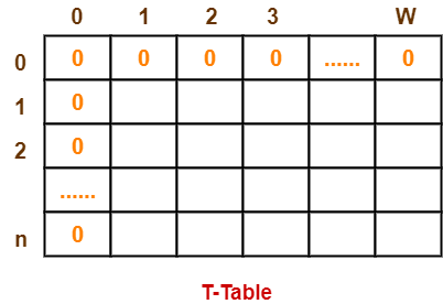
  • Draw a table say ‘T’ with (n+1) number of rows and (w+1) number of columns.
  • Fill all the boxes of 0th row and 0th column with zeroes as shown-


Step-02:


Start filling the table row wise top to bottom from left to right.

Use the following formula-

T (i , j) = max { T ( i-1 , j ) , valuei + T( i-1 , j – weight) }


Here, T(i , j) = maximum value of the selected items if we can take items 1 to i and have weight restrictions of j.


  • This step leads to completely filling the table.
  • Then, value of the last box represents the maximum possible value that can be put into the knapsack.


Step-03:


To identify the items that must be put into the knapsack to obtain that maximum profit,

  • Consider the last column of the table.
  • Start scanning the entries from bottom to top.
  • On encountering an entry whose value is not same as the value stored in the entry immediately above it, mark the row label of that entry.
  • After all the entries are scanned, the marked labels represent the items that must be put into the knapsack.


Time Complexity-


  • Each entry of the table requires constant time θ(1) for its computation.
  • It takes θ(nw) time to fill (n+1)(w+1) table entries.
  • It takes θ(n) time for tracing the solution since tracing process traces the n rows.
  • Thus, overall θ(nw) time is taken to solve 0/1 knapsack problem using dynamic programming.


PRACTICE PROBLEM BASED ON 0/1 KNAPSACK PROBLEM-


Problem-


For the given set of items and knapsack capacity = 5 kg, find the optimal solution for the 0/1 knapsack problem making use of dynamic programming approach.


Item Weight Value
1 2 3
2 3 4
3 4 5
4 5 6


OR


Find the optimal solution for the 0/1 knapsack problem making use of dynamic programming approach. Consider-

n = 4

w = 5 kg

(w1, w2, w3, w4) = (2, 3, 4, 5)

(b1, b2, b3, b4) = (3, 4, 5, 6)


OR


A thief enters a house for robbing it. He can carry a maximal weight of 5 kg into his bag. There are 4 items in the house with the following weights and values. What items should thief take if he either takes the item completely or leaves it completely?


Item Weight (kg) Value ($)
Mirror 2 3
Silver nugget 3 4
Painting 4 5
Vase 5 6


Solution-


Given-


  • Knapsack capacity (w) = 5 kg
  • Number of items (n) = 4


Step-01:


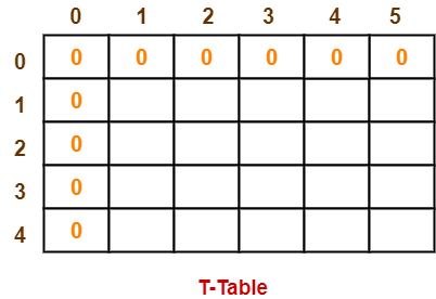
  • Draw a table say ‘T’ with (n+1) = 4 + 1 = 5 number of rows and (w+1) = 5 + 1 = 6 number of columns.
  • Fill all the boxes of 0th row and 0th column with 0.


Step-02:


Start filling the table row wise top to bottom from left to right using the formula-

T (i , j) = max { T ( i-1 , j ) , valuei + T( i-1 , j – weight) }


Finding T(1,1)-


We have,

  • i = 1
  • j = 1
  • (value)i = (value)1 = 3
  • (weight)i = (weight)1 = 2


Substituting the values, we get-

T(1,1) = max { T(1-1 , 1) , 3 + T(1-1 , 1-2) }

T(1,1) = max { T(0,1) , 3 + T(0,-1) }

T(1,1) = T(0,1)             { Ignore T(0,-1) }

T(1,1) = 0


Finding T(1,2)-


We have,

  • i = 1
  • j = 2
  • (value)i = (value)1 = 3
  • (weight)i = (weight)1 = 2


Substituting the values, we get-

T(1,2) = max { T(1-1 , 2) , 3 + T(1-1 , 2-2) }

T(1,2) = max { T(0,2) , 3 + T(0,0) }

T(1,2) = max {0 , 3+0}

T(1,2) = 3


Finding T(1,3)-


We have,

  • i = 1
  • j = 3
  • (value)i = (value)1 = 3
  • (weight)i = (weight)1 = 2


Substituting the values, we get-

T(1,3) = max { T(1-1 , 3) , 3 + T(1-1 , 3-2) }

T(1,3) = max { T(0,3) , 3 + T(0,1) }

T(1,3) = max {0 , 3+0}

T(1,3) = 3


Finding T(1,4)-


We have,

  • i = 1
  • j = 4
  • (value)i = (value)1 = 3
  • (weight)i = (weight)1 = 2


Substituting the values, we get-

T(1,4) = max { T(1-1 , 4) , 3 + T(1-1 , 4-2) }

T(1,4) = max { T(0,4) , 3 + T(0,2) }

T(1,4) = max {0 , 3+0}

T(1,4) = 3


Finding T(1,5)-


We have,

  • i = 1
  • j = 5
  • (value)i = (value)1 = 3
  • (weight)i = (weight)1 = 2


Substituting the values, we get-

T(1,5) = max { T(1-1 , 5) , 3 + T(1-1 , 5-2) }

T(1,5) = max { T(0,5) , 3 + T(0,3) }

T(1,5) = max {0 , 3+0}

T(1,5) = 3


Finding T(2,1)-


We have,

  • i = 2
  • j = 1
  • (value)i = (value)2 = 4
  • (weight)i = (weight)2 = 3


Substituting the values, we get-

T(2,1) = max { T(2-1 , 1) , 4 + T(2-1 , 1-3) }

T(2,1) = max { T(1,1) , 4 + T(1,-2) }

T(2,1) = T(1,1)           { Ignore T(1,-2) }

T(2,1) = 0


Finding T(2,2)-


We have,

  • i = 2
  • j = 2
  • (value)i = (value)2 = 4
  • (weight)i = (weight)2 = 3


Substituting the values, we get-

T(2,2) = max { T(2-1 , 2) , 4 + T(2-1 , 2-3) }

T(2,2) = max { T(1,2) , 4 + T(1,-1) }

T(2,2) = T(1,2)           { Ignore T(1,-1) }

T(2,2) = 3


Finding T(2,3)-


We have,

  • i = 2
  • j = 3
  • (value)i = (value)2 = 4
  • (weight)i = (weight)2 = 3


Substituting the values, we get-

T(2,3) = max { T(2-1 , 3) , 4 + T(2-1 , 3-3) }

T(2,3) = max { T(1,3) , 4 + T(1,0) }

T(2,3) = max { 3 , 4+0 }

T(2,3) = 4


Finding T(2,4)-


We have,

  • i = 2
  • j = 4
  • (value)i = (value)2 = 4
  • (weight)i = (weight)2 = 3


Substituting the values, we get-

T(2,4) = max { T(2-1 , 4) , 4 + T(2-1 , 4-3) }

T(2,4) = max { T(1,4) , 4 + T(1,1) }

T(2,4) = max { 3 , 4+0 }

T(2,4) = 4


Finding T(2,5)-


We have,

  • i = 2
  • j = 5
  • (value)i = (value)2 = 4
  • (weight)i = (weight)2 = 3


Substituting the values, we get-

T(2,5) = max { T(2-1 , 5) , 4 + T(2-1 , 5-3) }

T(2,5) = max { T(1,5) , 4 + T(1,2) }

T(2,5) = max { 3 , 4+3 }

T(2,5) = 7


Similarly, compute all the entries.

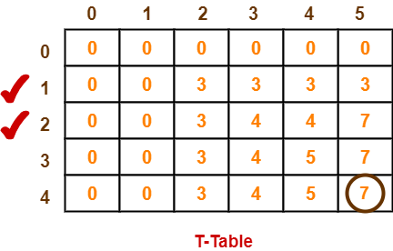
After all the entries are computed and filled in the table, we get the following table-


  • The last entry represents the maximum possible value that can be put into the knapsack.
  • So, maximum possible value that can be put into the knapsack = 7.


Identifying Items To Be Put Into Knapsack-


Following Step-04,

  • We mark the rows labelled “1” and “2”.
  • Thus, items that must be put into the knapsack to obtain the maximum value 7 are-

Item-1 and Item-2


To gain better understanding about 0/1 Knapsack Problem,

Watch this Video Lecture


Next Article- Travelling Salesman Problem


Get more notes and other study material of Design and Analysis of Algorithms.

Watch video lectures by visiting our YouTube channel LearnVidFun.
Fractional Knapsack Problem | Greedy Method | Example

Knapsack Problem-


You are given the following-

  • A knapsack (kind of shoulder bag) with limited weight capacity.
  • Few items each having some weight and value.


The problem states-

Which items should be placed into the knapsack such that-

  • The value or profit obtained by putting the items into the knapsack is maximum.
  • And the weight limit of the knapsack does not exceed.


Knapsack Problem Variants-


Knapsack problem has the following two variants-

  1. Fractional Knapsack Problem
  2. 0/1 Knapsack Problem


In this article, we will discuss about Fractional Knapsack Problem.


Fractional Knapsack Problem-


In Fractional Knapsack Problem,

  • As the name suggests, items are divisible here.
  • We can even put the fraction of any item into the knapsack if taking the complete item is not possible.
  • It is solved using Greedy Method.


Also Read- 0/1 Knapsack Problem


Fractional Knapsack Problem Using Greedy Method-


Fractional knapsack problem is solved using greedy method in the following steps-


Step-01:


For each item, compute its value / weight ratio.


Step-02:


Arrange all the items in decreasing order of their value / weight ratio.


Step-03:


Start putting the items into the knapsack beginning from the item with the highest ratio.

Put as many items as you can into the knapsack.


Time Complexity-


  • The main time taking step is the sorting of all items in decreasing order of their value / weight ratio.
  • If the items are already arranged in the required order, then while loop takes O(n) time.
  • The average time complexity of Quick Sort is O(nlogn).
  • Therefore, total time taken including the sort is O(nlogn).


PRACTICE PROBLEM BASED ON FRACTIONAL KNAPSACK PROBLEM-


Problem-


For the given set of items and knapsack capacity = 60 kg, find the optimal solution for the fractional knapsack problem making use of greedy approach.


Item Weight Value
1 5 30
2 10 40
3 15 45
4 22 77
5 25 90


OR


Find the optimal solution for the fractional knapsack problem making use of greedy approach. Consider-

n = 5

w = 60 kg

(w1, w2, w3, w4, w5) = (5, 10, 15, 22, 25)

(b1, b2, b3, b4, b5) = (30, 40, 45, 77, 90)


OR


A thief enters a house for robbing it. He can carry a maximal weight of 60 kg into his bag. There are 5 items in the house with the following weights and values. What items should thief take if he can even take the fraction of any item with him?


Item Weight Value
1 5 30
2 10 40
3 15 45
4 22 77
5 25 90


Solution-


Step-01:


Compute the value / weight ratio for each item-


Items Weight Value Ratio
1 5 30 6
2 10 40 4
3 15 45 3
4 22 77 3.5
5 25 90 3.6


Step-02:


Sort all the items in decreasing order of their value / weight ratio-


I1          I2          I5          I4          I3

(6)       (4)        (3.6)      (3.5)       (3)


Step-03:


Start filling the knapsack by putting the items into it one by one.


Knapsack Weight Items in Knapsack Cost
60 Ø 0
55 I1 30
45 I1, I2 70
20 I1, I2, I5 160


Now,

  • Knapsack weight left to be filled is 20 kg but item-4 has a weight of 22 kg.
  • Since in fractional knapsack problem, even the fraction of any item can be taken.
  • So, knapsack will contain the following items-

< I1 , I2 , I5 , (20/22) I4 >


Total cost of the knapsack

= 160 + (20/27) x 77

= 160 + 70

= 230 units


Important Note-


Had the problem been a 0/1 knapsack problem, knapsack would contain the following items-

< I1 , I2 , I5 >

The knapsack’s total cost would be 160 units.


To gain better understanding about Fractional Knapsack Problem,

Watch this Video Lecture


Next Article- Job Sequencing With Deadlines


Get more notes and other study material of Design and Analysis of Algorithms.

Watch video lectures by visiting our YouTube channel LearnVidFun.