Tag: Data Structures and Algorithms

Open Addressing | Linear Probing | Collision

Collision Resolution Techniques-


Before you go through this article, make sure that you have gone through the previous article on Collision Resolution Techniques.


We have discussed-

  • Hashing is a well-known searching technique.
  • Collision occurs when hash value of the new key maps to an occupied bucket of the hash table.
  • Collision resolution techniques are classified as-
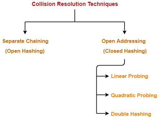


In this article, we will discuss about Open Addressing.


Open Addressing-


In open addressing,

  • Unlike separate chaining, all the keys are stored inside the hash table.
  • No key is stored outside the hash table.


Techniques used for open addressing are-

  • Linear Probing
  • Quadratic Probing
  • Double Hashing


Operations in Open Addressing-


Let us discuss how operations are performed in open addressing-


Insert Operation-


  • Hash function is used to compute the hash value for a key to be inserted.
  • Hash value is then used as an index to store the key in the hash table.


In case of collision,

  • Probing is performed until an empty bucket is found.
  • Once an empty bucket is found, the key is inserted.
  • Probing is performed in accordance with the technique used for open addressing.


Search Operation-


To search any particular key,

  • Its hash value is obtained using the hash function used.
  • Using the hash value, that bucket of the hash table is checked.
  • If the required key is found, the key is searched.
  • Otherwise, the subsequent buckets are checked until the required key or an empty bucket is found.
  • The empty bucket indicates that the key is not present in the hash table.


Delete Operation-


  • The key is first searched and then deleted.
  • After deleting the key, that particular bucket is marked as “deleted”.


NOTE-


  • During insertion, the buckets marked as “deleted” are treated like any other empty bucket.
  • During searching, the search is not terminated on encountering the bucket marked as “deleted”.
  • The search terminates only after the required key or an empty bucket is found.


Open Addressing Techniques-


Techniques used for open addressing are-


1. Linear Probing-


In linear probing,

  • When collision occurs, we linearly probe for the next bucket.
  • We keep probing until an empty bucket is found.


Advantage-


  • It is easy to compute.


Disadvantage-


  • The main problem with linear probing is clustering.
  • Many consecutive elements form groups.
  • Then, it takes time to search an element or to find an empty bucket.


Time Complexity-


Worst time to search an element in linear probing is O (table size).


This is because-

  • Even if there is only one element present and all other elements are deleted.
  • Then, “deleted” markers present in the hash table makes search the entire table.


2. Quadratic Probing-


In quadratic probing,

  • When collision occurs, we probe for i2‘th bucket in ith iteration.
  • We keep probing until an empty bucket is found.


3. Double Hashing-


In double hashing,

  • We use another hash function hash2(x) and look for i * hash2(x) bucket in ith iteration.
  • It requires more computation time as two hash functions need to be computed.


Comparison of Open Addressing Techniques-


Linear Probing
Quadratic Probing
Double Hashing
Primary Clustering
Yes No No
Secondary Clustering
Yes Yes No
Number of Probe Sequence
(m = size of table)
m m m2
Cache performance
Best Lies between the two Poor


Conclusions-


  • Linear Probing has the best cache performance but suffers from clustering.
  • Quadratic probing lies between the two in terms of cache performance and clustering.
  • Double caching has poor cache performance but no clustering.


Load Factor (α)-


Load factor (α) is defined as-


In open addressing, the value of load factor always lie between 0 and 1.


This is because-

  • In open addressing, all the keys are stored inside the hash table.
  • So, size of the table is always greater or at least equal to the number of keys stored in the table.


PRACTICE PROBLEM BASED ON OPEN ADDRESSING-


Problem-


Using the hash function ‘key mod 7’, insert the following sequence of keys in the hash table-

50, 700, 76, 85, 92, 73 and 101


Use linear probing technique for collision resolution.


Solution-


The given sequence of keys will be inserted in the hash table as-


Step-01:


  • Draw an empty hash table.
  • For the given hash function, the possible range of hash values is [0, 6].
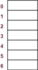
  • So, draw an empty hash table consisting of 7 buckets as-


Step-02:


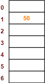
  • Insert the given keys in the hash table one by one.
  • The first key to be inserted in the hash table = 50.
  • Bucket of the hash table to which key 50 maps = 50 mod 7 = 1.
  • So, key 50 will be inserted in bucket-1 of the hash table as-


Step-03:


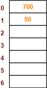
  • The next key to be inserted in the hash table = 700.
  • Bucket of the hash table to which key 700 maps = 700 mod 7 = 0.
  • So, key 700 will be inserted in bucket-0 of the hash table as-


Step-04:


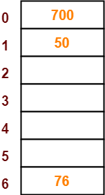
  • The next key to be inserted in the hash table = 76.
  • Bucket of the hash table to which key 76 maps = 76 mod 7 = 6.
  • So, key 76 will be inserted in bucket-6 of the hash table as-


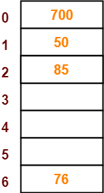
Step-05:


  • The next key to be inserted in the hash table = 85.
  • Bucket of the hash table to which key 85 maps = 85 mod 7 = 1.
  • Since bucket-1 is already occupied, so collision occurs.
  • To handle the collision, linear probing technique keeps probing linearly until an empty bucket is found.
  • The first empty bucket is bucket-2.
  • So, key 85 will be inserted in bucket-2 of the hash table as-


Step-06:


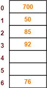
  • The next key to be inserted in the hash table = 92.
  • Bucket of the hash table to which key 92 maps = 92 mod 7 = 1.
  • Since bucket-1 is already occupied, so collision occurs.
  • To handle the collision, linear probing technique keeps probing linearly until an empty bucket is found.
  • The first empty bucket is bucket-3.
  • So, key 92 will be inserted in bucket-3 of the hash table as-


Step-07:


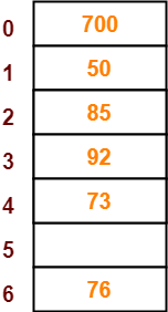
  • The next key to be inserted in the hash table = 73.
  • Bucket of the hash table to which key 73 maps = 73 mod 7 = 3.
  • Since bucket-3 is already occupied, so collision occurs.
  • To handle the collision, linear probing technique keeps probing linearly until an empty bucket is found.
  • The first empty bucket is bucket-4.
  • So, key 73 will be inserted in bucket-4 of the hash table as-


Step-08:


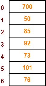
  • The next key to be inserted in the hash table = 101.
  • Bucket of the hash table to which key 101 maps = 101 mod 7 = 3.
  • Since bucket-3 is already occupied, so collision occurs.
  • To handle the collision, linear probing technique keeps probing linearly until an empty bucket is found.
  • The first empty bucket is bucket-5.
  • So, key 101 will be inserted in bucket-5 of the hash table as-


To gain better understanding about Open Addressing,

Watch this Video Lecture


Next Article- Separate Chaining Vs Open Addressing


Get more notes and other study material of Data Structures.

Watch video lectures by visiting our YouTube channel LearnVidFun.

Separate Chaining | Collision Resolution Techniques

Hashing in Data Structure-


Before you go through this article, make sure that you have gone through the previous article on Hashing.


We have discussed-

  • Hashing is a well-known searching technique.
  • It minimizes the number of comparisons while performing the search.
  • It completes the search with constant time complexity O(1).


In this article, we will discuss about Collisions in Hashing.


Collision in Hashing-


In hashing,

  • Hash function is used to compute the hash value for a key.
  • Hash value is then used as an index to store the key in the hash table.
  • Hash function may return the same hash value for two or more keys.


When the hash value of a key maps to an already occupied bucket of the hash table,

it is called as a Collision.


Collision Resolution Techniques-


Collision Resolution Techniques are the techniques used for resolving or handling the collision.


Collision resolution techniques are classified as-


  1. Separate Chaining
  2. Open Addressing


In this article, we will discuss about separate chaining.


Separate Chaining-


To handle the collision,

  • This technique creates a linked list to the slot for which collision occurs.
  • The new key is then inserted in the linked list.
  • These linked lists to the slots appear like chains.
  • That is why, this technique is called as separate chaining.


Time Complexity-


For Searching-


  • In worst case, all the keys might map to the same bucket of the hash table.
  • In such a case, all the keys will be present in a single linked list.
  • Sequential search will have to be performed on the linked list to perform the search.
  • So, time taken for searching in worst case is O(n).


For Deletion-


  • In worst case, the key might have to be searched first and then deleted.
  • In worst case, time taken for searching is O(n).
  • So, time taken for deletion in worst case is O(n).


Load Factor (α)-


Load factor (α) is defined as-


If Load factor (α) = constant, then time complexity of Insert, Search, Delete = Θ(1)


PRACTICE PROBLEM BASED ON SEPARATE CHAINING-


Problem-


Using the hash function ‘key mod 7’, insert the following sequence of keys in the hash table-

50, 700, 76, 85, 92, 73 and 101


Use separate chaining technique for collision resolution.


Solution-


The given sequence of keys will be inserted in the hash table as-


Step-01:


  • Draw an empty hash table.
  • For the given hash function, the possible range of hash values is [0, 6].
  • So, draw an empty hash table consisting of 7 buckets as-


Step-02:


  • Insert the given keys in the hash table one by one.
  • The first key to be inserted in the hash table = 50.
  • Bucket of the hash table to which key 50 maps = 50 mod 7 = 1.
  • So, key 50 will be inserted in bucket-1 of the hash table as-


Step-03:


  • The next key to be inserted in the hash table = 700.
  • Bucket of the hash table to which key 700 maps = 700 mod 7 = 0.
  • So, key 700 will be inserted in bucket-0 of the hash table as-


Step-04:


  • The next key to be inserted in the hash table = 76.
  • Bucket of the hash table to which key 76 maps = 76 mod 7 = 6.
  • So, key 76 will be inserted in bucket-6 of the hash table as-


Step-05:


  • The next key to be inserted in the hash table = 85.
  • Bucket of the hash table to which key 85 maps = 85 mod 7 = 1.
  • Since bucket-1 is already occupied, so collision occurs.
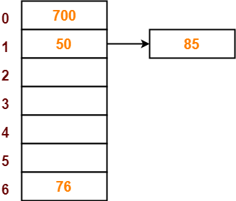
  • Separate chaining handles the collision by creating a linked list to bucket-1.
  • So, key 85 will be inserted in bucket-1 of the hash table as-


Step-06:


  • The next key to be inserted in the hash table = 92.
  • Bucket of the hash table to which key 92 maps = 92 mod 7 = 1.
  • Since bucket-1 is already occupied, so collision occurs.
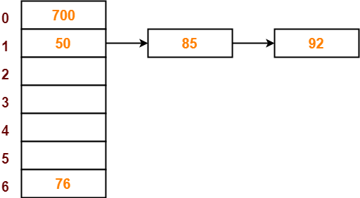
  • Separate chaining handles the collision by creating a linked list to bucket-1.
  • So, key 92 will be inserted in bucket-1 of the hash table as-


Step-07:


  • The next key to be inserted in the hash table = 73.
  • Bucket of the hash table to which key 73 maps = 73 mod 7 = 3.
  • So, key 73 will be inserted in bucket-3 of the hash table as-


Step-08:


  • The next key to be inserted in the hash table = 101.
  • Bucket of the hash table to which key 101 maps = 101 mod 7 = 3.
  • Since bucket-3 is already occupied, so collision occurs.
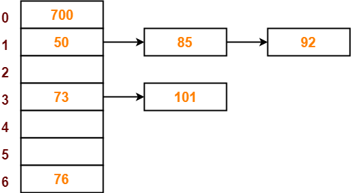
  • Separate chaining handles the collision by creating a linked list to bucket-3.
  • So, key 101 will be inserted in bucket-3 of the hash table as-


To gain better understanding about Separate Chaining,

Watch this Video Lecture


Next Article- Open Addressing


Get more notes and other study material of Data Structures.

Watch video lectures by visiting our YouTube channel LearnVidFun.
Hashing in Data Structure | Hash Functions

Searching Techniques-


In data structures,

  • There are several searching techniques like linear search, binary search, search trees etc.
  • In these techniques, time taken to search any particular element depends on the total number of elements.


Example-


  • Linear Search takes O(n) time to perform the search in unsorted arrays consisting of n elements.
  • Binary Search takes O(logn) time to perform the search in sorted arrays consisting of n elements.
  • It takes O(logn) time to perform the search in Binary Search Tree consisting of n elements.


Drawback-


The main drawback of these techniques is-

  • As the number of elements increases, time taken to perform the search also increases.
  • This becomes problematic when total number of elements become too large.


Hashing in Data Structure-


In data structures,

  • Hashing is a well-known technique to search any particular element among several elements.
  • It minimizes the number of comparisons while performing the search.


Advantage-


Unlike other searching techniques,

  • Hashing is extremely efficient.
  • The time taken by it to perform the search does not depend upon the total number of elements.
  • It completes the search with constant time complexity O(1).


Hashing Mechanism-


In hashing,

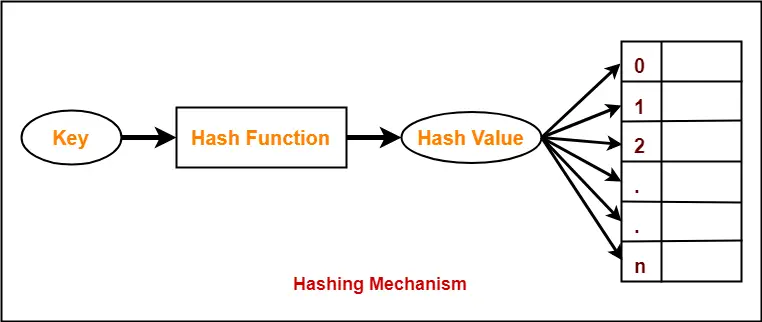
  • An array data structure called as Hash table is used to store the data items.
  • Based on the hash key value, data items are inserted into the hash table.


Hash Key Value-


  • Hash key value is a special value that serves as an index for a data item.
  • It indicates where the data item should be be stored in the hash table.
  • Hash key value is generated using a hash function.


Hash Function-


Hash function is a function that maps any big number or string to a small integer value.


  • Hash function takes the data item as an input and returns a small integer value as an output.
  • The small integer value is called as a hash value.
  • Hash value of the data item is then used as an index for storing it into the hash table.


Types of Hash Functions-


There are various types of hash functions available such as-

  1. Mid Square Hash Function
  2. Division Hash Function
  3. Folding Hash Function etc


It depends on the user which hash function he wants to use.


Properties of Hash Function-


The properties of a good hash function are-

  • It is efficiently computable.
  • It minimizes the number of collisions.
  • It distributes the keys uniformly over the table.


To gain better understanding about Hashing in Data Structures,

Watch this Video Lecture


Next Article- Collision in Hashing


Get more notes and other study material of Data Structures.

Watch video lectures by visiting our YouTube channel LearnVidFun.
Job Sequencing With Deadlines | Algorithm | Example

Job Sequencing With Deadlines-


The sequencing of jobs on a single processor with deadline constraints is called as Job Sequencing with Deadlines.


Here-

  • You are given a set of jobs.
  • Each job has a defined deadline and some profit associated with it.
  • The profit of a job is given only when that job is completed within its deadline.
  • Only one processor is available for processing all the jobs.
  • Processor takes one unit of time to complete a job.


The problem states-

“How can the total profit be maximized if only one job can be completed at a time?”


Approach to Solution-


  • A feasible solution would be a subset of jobs where each job of the subset gets completed within its deadline.
  • Value of the feasible solution would be the sum of profit of all the jobs contained in the subset.
  • An optimal solution of the problem would be a feasible solution which gives the maximum profit.


Greedy Algorithm-


Greedy Algorithm is adopted to determine how the next job is selected for an optimal solution.

The greedy algorithm described below always gives an optimal solution to the job sequencing problem-


Step-01:


  • Sort all the given jobs in decreasing order of their profit.


Step-02:


  • Check the value of maximum deadline.
  • Draw a Gantt chart where maximum time on Gantt chart is the value of maximum deadline.


Step-03:


  • Pick up the jobs one by one.
  • Put the job on Gantt chart as far as possible from 0 ensuring that the job gets completed before its deadline.


PRACTICE PROBLEM BASED ON JOB SEQUENCING WITH DEADLINES-


Problem-


Given the jobs, their deadlines and associated profits as shown-


Jobs J1 J2 J3 J4 J5 J6
Deadlines 5 3 3 2 4 2
Profits 200 180 190 300 120 100


Answer the following questions-

  1. Write the optimal schedule that gives maximum profit.
  2. Are all the jobs completed in the optimal schedule?
  3. What is the maximum earned profit?


Solution-


Step-01:


Sort all the given jobs in decreasing order of their profit-


Jobs J4 J1 J3 J2 J5 J6
Deadlines 2 5 3 3 4 2
Profits 300 200 190 180 120 100


Step-02:


Value of maximum deadline = 5.

So, draw a Gantt chart with maximum time on Gantt chart = 5 units as shown-


Now,

  • We take each job one by one in the order they appear in Step-01.
  • We place the job on Gantt chart as far as possible from 0.


Step-03:


  • We take job J4.
  • Since its deadline is 2, so we place it in the first empty cell before deadline 2 as-


Step-04:


  • We take job J1.
  • Since its deadline is 5, so we place it in the first empty cell before deadline 5 as-


Step-05:


  • We take job J3.
  • Since its deadline is 3, so we place it in the first empty cell before deadline 3 as-


Step-06:


  • We take job J2.
  • Since its deadline is 3, so we place it in the first empty cell before deadline 3.
  • Since the second and third cells are already filled, so we place job J2 in the first cell as-


Step-07:


  • Now, we take job J5.
  • Since its deadline is 4, so we place it in the first empty cell before deadline 4 as-


Now,

  • The only job left is job J6 whose deadline is 2.
  • All the slots before deadline 2 are already occupied.
  • Thus, job J6 can not be completed.


Now, the given questions may be answered as-


Part-01:


The optimal schedule is-

J2  , J4 , J3 , J5 , J1

This is the required order in which the jobs must be completed in order to obtain the maximum profit.


Part-02:


  • All the jobs are not completed in optimal schedule.
  • This is because job J6 could not be completed within its deadline.


Part-03:


Maximum earned profit

= Sum of profit of all the jobs in optimal schedule

= Profit of job J2 + Profit of job J4 + Profit of job J3 + Profit of job J5 + Profit of job J1

= 180 + 300 + 190 + 120 + 200

= 990 units


To gain better understanding about Job Sequencing With Deadlines,

Watch this Video Lecture


Next Article- Huffman Coding


Get more notes and other study material of Design and Analysis of Algorithms.

Watch video lectures by visiting our YouTube channel LearnVidFun.
Travelling Salesman Problem | Branch & Bound

Travelling Salesman Problem-


You are given-

  • A set of some cities
  • Distance between every pair of cities


Travelling Salesman Problem states-

  • A salesman has to visit every city exactly once.
  • He has to come back to the city from where he starts his journey.
  • What is the shortest possible route that the salesman must follow to complete his tour?


Example-


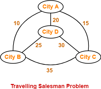
The following graph shows a set of cities and distance between every pair of cities-


If salesman starting city is A, then a TSP tour in the graph is-

A → B → D → C → A


Cost of the tour

= 10 + 25 + 30 + 15

= 80 units


In this article, we will discuss how to solve travelling salesman problem using branch and bound approach with example.


PRACTICE PROBLEM BASED ON TRAVELLING SALESMAN PROBLEM USING BRANCH AND BOUND APPROACH-


Problem-


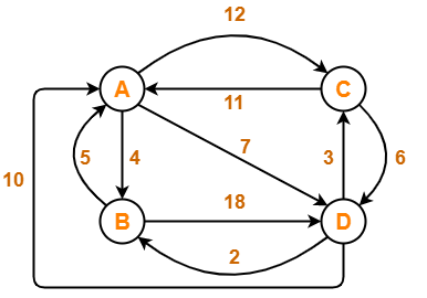
Solve Travelling Salesman Problem using Branch and Bound Algorithm in the following graph-


Solution-


Step-01:


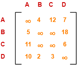
Write the initial cost matrix and reduce it-


Rules

  • To reduce a matrix, perform the row reduction and column reduction of the matrix separately.
  • A row or a column is said to be reduced if it contains at least one entry ‘0’ in it.


Row Reduction-


Consider the rows of above matrix one by one.


If the row already contains an entry ‘0’, then-

  • There is no need to reduce that row.


If the row does not contains an entry ‘0’, then-

  • Reduce that particular row.
  • Select the least value element from that row.
  • Subtract that element from each element of that row.
  • This will create an entry ‘0’ in that row, thus reducing that row.


Following this, we have-

  • Reduce the elements of row-1 by 4.
  • Reduce the elements of row-2 by 5.
  • Reduce the elements of row-3 by 6.
  • Reduce the elements of row-4 by 2.


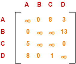
Performing this, we obtain the following row-reduced matrix-


Column Reduction-


Consider the columns of above row-reduced matrix one by one.


If the column already contains an entry ‘0’, then-

  • There is no need to reduce that column.


If the column does not contains an entry ‘0’, then-

  • Reduce that particular column.
  • Select the least value element from that column.
  • Subtract that element from each element of that column.
  • This will create an entry ‘0’ in that column, thus reducing that column.


Following this, we have-

  • There is no need to reduce column-1.
  • There is no need to reduce column-2.
  • Reduce the elements of column-3 by 1.
  • There is no need to reduce column-4.


Performing this, we obtain the following column-reduced matrix-


Finally, the initial distance matrix is completely reduced.

Now, we calculate the cost of node-1 by adding all the reduction elements.


Cost(1)

= Sum of all reduction elements

= 4 + 5 + 6 + 2 + 1

= 18


Step-02:


  • We consider all other vertices one by one.
  • We select the best vertex where we can land upon to minimize the tour cost.


Choosing To Go To Vertex-B: Node-2 (Path A → B)


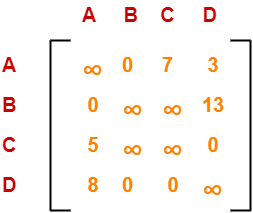
  • From the reduced matrix of step-01, M[A,B] = 0
  • Set row-A and column-B to 
  • Set M[B,A] = 


Now, resulting cost matrix is-


Now,

  • We reduce this matrix.
  • Then, we find out the cost of node-02.


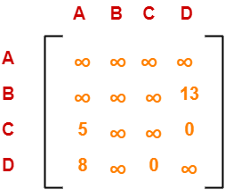
Row Reduction-


  • We can not reduce row-1 as all its elements are ∞.
  • Reduce all the elements of row-2 by 13.
  • There is no need to reduce row-3.
  • There is no need to reduce row-4.


Performing this, we obtain the following row-reduced matrix-


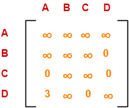
Column Reduction-


  • Reduce the elements of column-1 by 5.
  • We can not reduce column-2 as all its elements are ∞.
  • There is no need to reduce column-3.
  • There is no need to reduce column-4.


Performing this, we obtain the following column-reduced matrix-


Finally, the matrix is completely reduced.

Now, we calculate the cost of node-2.


Cost(2)

= Cost(1) + Sum of reduction elements + M[A,B]

= 18 + (13 + 5) + 0

= 36


Choosing To Go To Vertex-C: Node-3 (Path A → C)


  • From the reduced matrix of step-01, M[A,C] = 7
  • Set row-A and column-C to 
  • Set M[C,A] = 


Now, resulting cost matrix is-


Now,

  • We reduce this matrix.
  • Then, we find out the cost of node-03.


Row Reduction-


  • We can not reduce row-1 as all its elements are ∞.
  • There is no need to reduce row-2.
  • There is no need to reduce row-3.
  • There is no need to reduce row-4.


Thus, the matrix is already row-reduced.


Column Reduction-


  • There is no need to reduce column-1.
  • There is no need to reduce column-2.
  • We can not reduce column-3 as all its elements are ∞.
  • There is no need to reduce column-4.


Thus, the matrix is already column reduced.

Finally, the matrix is completely reduced.

Now, we calculate the cost of node-3.


Cost(3)

= Cost(1) + Sum of reduction elements + M[A,C]

= 18 + 0 + 7

= 25


Choosing To Go To Vertex-D: Node-4 (Path A → D)


  • From the reduced matrix of step-01, M[A,D] = 3
  • Set row-A and column-D to 
  • Set M[D,A] = 


Now, resulting cost matrix is-


Now,

  • We reduce this matrix.
  • Then, we find out the cost of node-04.


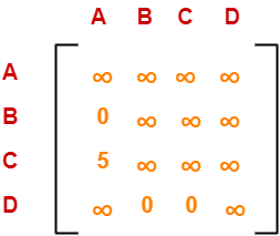
Row Reduction-


  • We can not reduce row-1 as all its elements are ∞.
  • There is no need to reduce row-2.
  • Reduce all the elements of row-3 by 5.
  • There is no need to reduce row-4.


Performing this, we obtain the following row-reduced matrix-


Column Reduction-


  • There is no need to reduce column-1.
  • There is no need to reduce column-2.
  • There is no need to reduce column-3.
  • We can not reduce column-4 as all its elements are ∞.


Thus, the matrix is already column-reduced.

Finally, the matrix is completely reduced.

Now, we calculate the cost of node-4.


Cost(4)

= Cost(1) + Sum of reduction elements + M[A,D]

= 18 + 5 + 3

= 26


Thus, we have-

  • Cost(2) = 36 (for Path A → B)
  • Cost(3) = 25 (for Path A → C)
  • Cost(4) = 26 (for Path A → D)


We choose the node with the lowest cost.

Since cost for node-3 is lowest, so we prefer to visit node-3.

Thus, we choose node-3 i.e. path A → C.


Step-03:


We explore the vertices B and D from node-3.

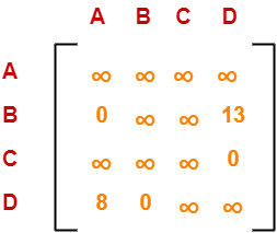
We now start from the cost matrix at node-3 which is-


Cost(3) = 25


Choosing To Go To Vertex-B: Node-5 (Path A → C → B)


  • From the reduced matrix of step-02, M[C,B] = 
  • Set row-C and column-B to 
  • Set M[B,A] = 


Now, resulting cost matrix is-


Now,

  • We reduce this matrix.
  • Then, we find out the cost of node-5.


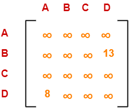
Row Reduction-


  • We can not reduce row-1 as all its elements are ∞.
  • Reduce all the elements of row-2 by 13.
  • We can not reduce row-3 as all its elements are ∞.
  • Reduce all the elements of row-4 by 8.


Performing this, we obtain the following row-reduced matrix-


Column Reduction-


  • There is no need to reduce column-1.
  • We can not reduce column-2 as all its elements are ∞.
  • We can not reduce column-3 as all its elements are ∞.
  • There is no need to reduce column-4.


Thus, the matrix is already column reduced.

Finally, the matrix is completely reduced.

Now, we calculate the cost of node-5.


Cost(5)

= cost(3) + Sum of reduction elements + M[C,B]

= 25 + (13 + 8) +

=


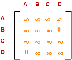
Choosing To Go To Vertex-D: Node-6 (Path A → C → D)


  • From the reduced matrix of step-02, M[C,D] = 
  • Set row-C and column-D to 
  • Set M[D,A] = 


Now, resulting cost matrix is-


Now,

  • We reduce this matrix.
  • Then, we find out the cost of node-6.


Row Reduction-


  • We can not reduce row-1 as all its elements are ∞.
  • There is no need to reduce row-2.
  • We can not reduce row-3 as all its elements are ∞.
  • We can not reduce row-4 as all its elements are ∞.


Thus, the matrix is already row reduced.


Column Reduction-


  • There is no need to reduce column-1.
  • We can not reduce column-2 as all its elements are ∞.
  • We can not reduce column-3 as all its elements are ∞.
  • We can not reduce column-4 as all its elements are ∞.


Thus, the matrix is already column reduced.

Finally, the matrix is completely reduced.

Now, we calculate the cost of node-6.


Cost(6)

= cost(3) + Sum of reduction elements + M[C,D]

= 25 + 0 + 0

= 25


Thus, we have-

  • Cost(5) =  (for Path A → C → B)
  • Cost(6) = 25 (for Path A → C → D)


We choose the node with the lowest cost.

Since cost for node-6 is lowest, so we prefer to visit node-6.

Thus, we choose node-6 i.e. path C → D.


Step-04:


We explore vertex B from node-6.

We start with the cost matrix at node-6 which is-


Cost(6) = 25


Choosing To Go To Vertex-B: Node-7 (Path A → C → D → B)


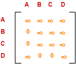
  • From the reduced matrix of step-03, M[D,B] = 0
  • Set row-D and column-B to 
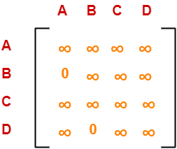
  • Set M[B,A] = 


Now, resulting cost matrix is-


Now,

  • We reduce this matrix.
  • Then, we find out the cost of node-7.


Row Reduction-


  • We can not reduce row-1 as all its elements are ∞.
  • We can not reduce row-2 as all its elements are ∞.
  • We can not reduce row-3 as all its elements are ∞.
  • We can not reduce row-4 as all its elements are ∞.


Column Reduction-


  • We can not reduce column-1 as all its elements are ∞.
  • We can not reduce column-2 as all its elements are ∞.
  • We can not reduce column-3 as all its elements are ∞.
  • We can not reduce column-4 as all its elements are ∞.


Thus, the matrix is already column reduced.

Finally, the matrix is completely reduced.

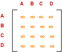
All the entries have become ∞.

Now, we calculate the cost of node-7.


Cost(7)

= cost(6) + Sum of reduction elements + M[D,B]

= 25 + 0 + 0

= 25


Thus,

  • Optimal path is: A → C → D → B → A
  • Cost of Optimal path = 25 units


To gain better understanding about Travelling Salesman Problem,

Watch this Video Lecture


Get more notes and other study material of Design and Analysis of Algorithms.

Watch video lectures by visiting our YouTube channel LearnVidFun.