Tag: Data Structures and Algorithms

Huffman Coding | Huffman Coding Example | Time Complexity

Huffman Coding-


  • Huffman Coding is a famous Greedy Algorithm.
  • It is used for the lossless compression of data.
  • It uses variable length encoding.
  • It assigns variable length code to all the characters.
  • The code length of a character depends on how frequently it occurs in the given text.
  • The character which occurs most frequently gets the smallest code.
  • The character which occurs least frequently gets the largest code.
  • It is also known as Huffman Encoding.


Prefix Rule-


  • Huffman Coding implements a rule known as a prefix rule.
  • This is to prevent the ambiguities while decoding.
  • It ensures that the code assigned to any character is not a prefix of the code assigned to any other character.


Major Steps in Huffman Coding-


There are two major steps in Huffman Coding-

  1. Building a Huffman Tree from the input characters.
  2. Assigning code to the characters by traversing the Huffman Tree.


Huffman Tree-


The steps involved in the construction of Huffman Tree are as follows-


Step-01:


  • Create a leaf node for each character of the text.
  • Leaf node of a character contains the occurring frequency of that character.


Step-02:


  • Arrange all the nodes in increasing order of their frequency value.


Step-03:


Considering the first two nodes having minimum frequency,

  • Create a new internal node.
  • The frequency of this new node is the sum of frequency of those two nodes.
  • Make the first node as a left child and the other node as a right child of the newly created node.


Step-04:


  • Keep repeating Step-02 and Step-03 until all the nodes form a single tree.
  • The tree finally obtained is the desired Huffman Tree.


Time Complexity-


The time complexity analysis of Huffman Coding is as follows-

  • extractMin( ) is called 2 x (n-1) times if there are n nodes.
  • As extractMin( ) calls minHeapify( ), it takes O(logn) time.


Thus, Overall time complexity of Huffman Coding becomes O(nlogn).

Here, n is the number of unique characters in the given text.


Important Formulas-


The following 2 formulas are important to solve the problems based on Huffman Coding-


Formula-01:


Formula-02:


Total number of bits in Huffman encoded message

= Total number of characters in the message x Average code length per character

= ∑ ( frequencyi x Code length)


PRACTICE PROBLEM BASED ON HUFFMAN CODING-


Problem-


A file contains the following characters with the frequencies as shown. If Huffman Coding is used for data compression, determine-

  1. Huffman Code for each character
  2. Average code length
  3. Length of Huffman encoded message (in bits)


Characters Frequencies
a 10
e 15
i 12
o 3
u 4
s 13
t 1


Solution-


First let us construct the Huffman Tree.

Huffman Tree is constructed in the following steps-


Step-01:


Step-02:


Step-03:
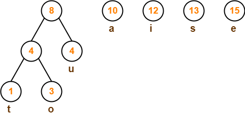


Step-04:
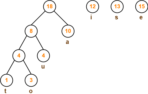


Step-05:
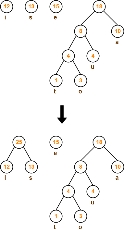


Step-06:
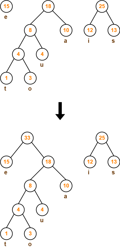


Step-07:
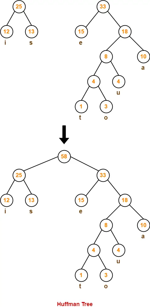


Now,

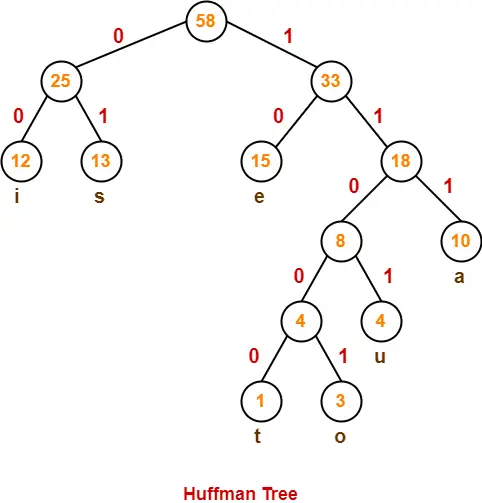
  • We assign weight to all the edges of the constructed Huffman Tree.
  • Let us assign weight ‘0’ to the left edges and weight ‘1’ to the right edges.


Rule

  • If you assign weight ‘0’ to the left edges, then assign weight ‘1’ to the right edges.
  • If you assign weight ‘1’ to the left edges, then assign weight ‘0’ to the right edges.
  • Any of the above two conventions may be followed.
  • But follow the same convention at the time of decoding that is adopted at the time of encoding.


After assigning weight to all the edges, the modified Huffman Tree is-


Now, let us answer each part of the given problem one by one-


1. Huffman Code For Characters-


To write Huffman Code for any character, traverse the Huffman Tree from root node to the leaf node of that character.

Following this rule, the Huffman Code for each character is-

  • a = 111
  • e = 10
  • i = 00
  • o = 11001
  • u = 1101
  • s = 01
  • t = 11000


From here, we can observe-

  • Characters occurring less frequently in the text are assigned the larger code.
  • Characters occurring more frequently in the text are assigned the smaller code.


2. Average Code Length-


Using formula-01, we have-

Average code length

= ∑ ( frequencyi x code lengthi ) / ∑ ( frequencyi )

= { (10 x 3) + (15 x 2) + (12 x 2) + (3 x 5) + (4 x 4) + (13 x 2) + (1 x 5) } / (10 + 15 + 12 + 3 + 4 + 13 + 1)

= 2.52


3. Length of Huffman Encoded Message-


Using formula-02, we have-

Total number of bits in Huffman encoded message

= Total number of characters in the message x Average code length per character

= 58 x 2.52

= 146.16

≅ 147 bits


To gain better understanding about Huffman Coding,

Watch this Video Lecture


To practice previous years GATE problems on Huffman Coding,

Watch this Video Lecture


Next Article- 0/1 Knapsack Problem


Get more notes and other study material of Design and Analysis of Algorithms.

Watch video lectures by visiting our YouTube channel LearnVidFun.
Breadth First Search Algorithm | BFS Example

Breadth First Search-


  • Breadth First Search or BFS is a graph traversal algorithm.
  • It is used for traversing or searching a graph in a systematic fashion.
  • BFS uses a strategy that searches in the graph in breadth first manner whenever possible.
  • Queue data structure is used in the implementation of breadth first search.


BFS Example-


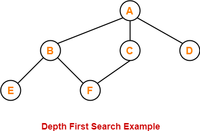
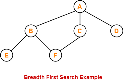
Consider the following graph-


The breadth first search traversal order of the above graph is-

A, B, C, D, E, F


Breadth First Search Algorithm-


BFS (V,E,s)


for each vertex v in V – {s}

do

color[v] ← WHITE

d[v] ← ∞

π[v] ← NIL

color[s] = GREY

d[s] ← 0

π[s] ← NIL

Q ← { }

ENQUEUE (Q,s)

While Q is non-empty

do v ← DEQUEUE (Q)

for each u adjacent to v

do if color[u] ← WHITE

then color[u] ← GREY

d[u] ← d[v] + 1

π[u] ← v

ENQUEUE (Q,u)

color[v] ← BLACK


Explanation-


The above breadth first search algorithm is explained in the following steps-


Step-01


Create and maintain 3 variables for each vertex of the graph.

For any vertex ‘v’ of the graph, these 3 variables are-


1. color[v]-


  • This variable represents the color of the vertex v at the given point of time.
  • The possible values of this variable are- WHITE, GREY and BLACK.
  • WHITE color of the vertex signifies that it has not been discovered yet.
  • GREY color of the vertex signifies that it has been discovered and it is being processed.
  • BLACK color of the vertex signifies that it has been completely processed.


2. Π[v]-


This variable represents the predecessor of vertex ‘v’.


3. d[v]-


This variable represents the distance of vertex v from the source vertex.


Step-02


For each vertex v of the graph except source vertex, initialize the variables as-

  • color[v] = WHITE
  • π[v] = NIL
  • d[v] = ∞


For source vertex S, initialize the variables as-

  • color[S] = GREY
  • π[S] = NIL
  • d[S] = 0


Step-03


Now, enqueue source vertex S in queue Q and repeat the following procedure until the queue Q becomes empty-

1. Dequeue vertex v from queue Q.

2. For all the adjacent white vertices u of vertex v,

do-

color[u] = GREY

d[u] = d[v] + 1

π[u] = v

Enqueue (Q,u)

3. Color vertex v to black.


BFS Time Complexity-


The total running time for Breadth First Search is O (V+E).


Also Read- Depth First Search


PRACTICE PROBLEM BASED ON BREADTH FIRST SEARCH-


Problem-


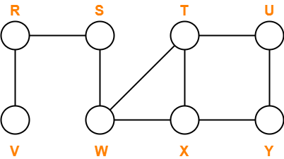
Traverse the following graph using Breadth First Search Technique-


Consider vertex S as the starting vertex.


Solution-


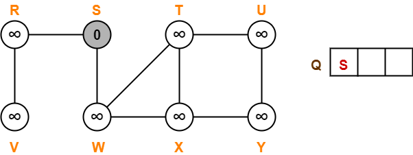
Step-01:


For all the vertices v except source vertex S of the graph, we initialize the variables as-

  • color[v] = WHITE
  • π[v] = NIL
  • d[v] = ∞


For source vertex S, we initialize the variables as-

  • color[S] = GREY
  • π[S] = NIL
  • d[S] = 0


We enqueue the source vertex S in the queue Q.


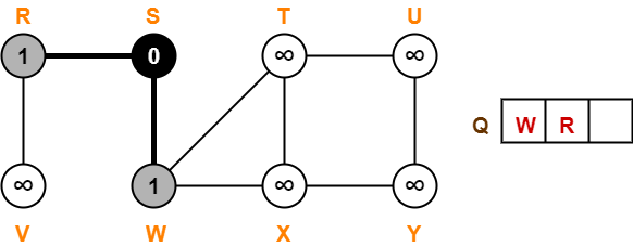
Step-02:


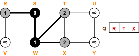
  • Dequeue vertex S from the queue Q
  • For all adjacent white vertices ‘v’ (vertices R and W) of vertex S, we do-


  1. color[v] = GREY
  2. d[v] = d[S] + 1 = 0 + 1 = 1
  3. π[v] = S
  4. Enqueue all adjacent white vertices of S in queue Q


  • color[S] = BLACK


Step-03:


  • Dequeue vertex W from the queue Q
  • For all adjacent white vertices ‘v’ (vertices T and X) of vertex W, we do-


  1. color[v] = GREY
  2. d[v] = d[W] + 1 = 1 + 1 = 2
  3. π[v] = W
  4. Enqueue all adjacent white vertices of W in queue Q


  • color[W] = BLACK


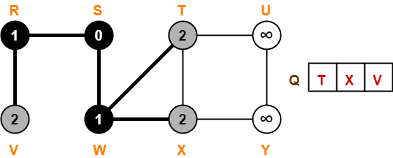
Step-04:


  • Dequeue vertex R from the queue Q
  • For all adjacent white vertices ‘v’ (vertex V) of vertex R, we do-


  1. color[v] = GREY
  2. d[v] = d[R] + 1 = 1 + 1 = 2
  3. π[v] = R
  4. Enqueue all adjacent white vertices of R in queue Q


  • color[R] = BLACK


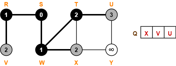
Step-05:


  • Dequeue vertex T from the queue Q
  • For all adjacent white vertices ‘v’ (vertex U) of vertex T, we do-


  1. color[v] = GREY
  2. d[v] = d[T] + 1 = 2 + 1 = 3
  3. π[v] = T
  4. Enqueue all adjacent white vertices of T in queue Q


  • color[T] = BLACK


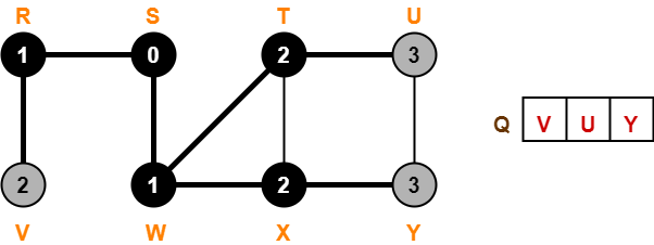
Step-06:


  • Dequeue vertex X from the queue Q
  • For all adjacent white vertices ‘v’ (vertex Y) of vertex X, we do-


  1. color[v] = GREY
  2. d[v] = d[X] + 1 = 2 + 1 = 3
  3. π[v] = X
  4. Enqueue all adjacent white vertices of X in queue Q


  • color[X] = BLACK


Step-07:


  • Dequeue vertex V from the queue Q
  • There are no adjacent white vertices to vertex V.
  • color[V] = BLACK


Step-08:


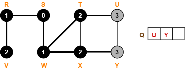
  • Dequeue vertex U from the queue Q
  • There are no adjacent white vertices to vertex U.
  • color[U] = BLACK


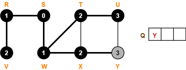
Step-09:


  • Dequeue vertex Y from the queue Q
  • There are no adjacent white vertices to vertex Y.
  • color[Y] = BLACK


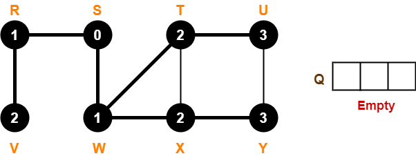
Since, all the vertices have turned black and the queue has got empty, so we stop.

This is how any given graph is traversed using Breadth First Search (BFS) technique.


To gain better understanding about Breadth First Search Algorithm,

Watch this Video Lecture


Next Article- Prim’s Algorithm


Get more notes and other study material of Design and Analysis of Algorithms.

Watch video lectures by visiting our YouTube channel LearnVidFun.
Depth First Search Algorithm | DFS Example

Depth First Search-


  • Depth First Search or DFS is a graph traversal algorithm.
  • It is used for traversing or searching a graph in a systematic fashion.
  • DFS uses a strategy that searches “deeper” in the graph whenever possible.
  • Stack data structure is used in the implementation of depth first search.


DFS Example-


Consider the following graph-


The depth first search traversal order of the above graph is-

A, B, E, F, C, D


Depth First Search Algorithm-


DFS (V,E)


for each vertex u in V[G]

do color[v] ← WHITE

π[v] ← NIL

time ← 0

for each vertex v in V[G]

do if color[v] ← WHITE

then Depth_First_Search(v)


Depth_First_Search (v)


color[v] ← GRAY

time ← time + 1

d[v] ← time

for each vertex u adjacent to v

do if color[u] ← WHITE

π[u] ← v

Depth_First_Search(u)

color[v] ← BLACK

time ← time + 1

f[v] ← time


Explanation-


The above depth first search algorithm is explained in the following steps-


Step-01


Create and maintain 4 variables for each vertex of the graph.

For any vertex ‘v’ of the graph, these 4 variables are-


1. color[v]-


  • This variable represents the color of the vertex ‘v’ at the given point of time.
  • The possible values of this variable are- WHITE, GREY and BLACK.
  • WHITE color of the vertex signifies that it has not been discovered yet.
  • GREY color of the vertex signifies that it has been discovered and it is being processed.
  • BLACK color of the vertex signifies that it has been completely processed.


2. Π[v]-


This variable represents the predecessor of vertex ‘v’.


3. d[v]-


This variable represents a timestamp when a vertex ‘v’ is discovered.


3. f[v]-


This variable represents a timestamp when the processing of vertex ‘v’ is completed.


Step-02


For each vertex of the graph, initialize the variables as-

  • color[v] = WHITE
  • π[v] = NIL
  • time = 0     (Global Variable acting as a timer)


Step-03


Repeat the following procedure until all the vertices of the graph become BLACK-

Consider any white vertex ‘v’ and call the following Depth_First_Search function on it.


Depth_First_Search (G,v)


1. color[v] = GRAY

2. time = time + 1

3. d[v] = time

4. For each adjacent WHITE vertex ‘u’ of ‘v’, set π[u] = v and call Depth_First_Search (G,u)

5. color[v] = BLACK

6. time = time + 1

7. f[v] = time


DFS Time Complexity-


The total running time for Depth First Search is θ (V+E).


Types of Edges in DFS-


After a DFS traversal of any graph G, all its edges can be put in one of the following 4 classes-


  1. Tree Edge
  2. Back Edge
  3. Forward Edge
  4. Cross Edge


1. Tree Edge-


  • A tree edge is an edge that is included in the DFS tree.


2. Back Edge-


An edge from a vertex ‘u’ to one of its ancestors ‘v’ is called as a back edge.

A self-loop is considered as a back edge.


A back edge is discovered when-

  • DFS tries to extend the visit from a vertex ‘u’ to vertex ‘v’
  • And vertex ‘v’ is found to be an ancestor of vertex ‘u’ and grey at that time.


3. Forward Edge-


An edge from a vertex ‘u’ to one of its descendants ‘v’ is called as a forward edge.


A forward edge is discovered when-

  • DFS tries to extend the visit from a vertex ‘u’ to a vertex ‘v’
  • And finds that color(v) = BLACK and d(v) > d(u).


4. Cross Edge-


An edge from a vertex ‘u’ to a vertex ‘v’ that is neither its ancestor nor its descendant is called as a cross edge.


A cross edge is discovered when-

  • DFS tries to extend the visit from a vertex ‘u’ to a vertex ‘v’
  • And finds that color(v) = BLACK and d(v) < d(u).


PRACTICE PROBLEM BASED ON DEPTH FIRST SEARCH-


Problem-


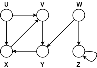
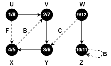
Compute the DFS tree for the graph given below-


Also, show the discovery and finishing time for each vertex and classify the edges.


Solution-


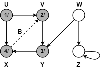
Initially for all the vertices of the graph, we set the variables as-

  • color[v] = WHITE
  • π[v] = NIL
  • time = 0 (Global)


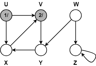
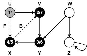
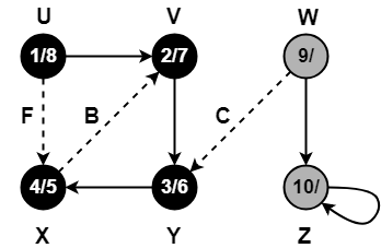
Let us start processing the graph from vertex U.


Step-01:


  • color[U] = GREY
  • time = 0 + 1 = 1
  • d[U] = 1


Step-02:


  • π[V] = U
  • color[V] = GREY
  • time = 1 + 1 = 2
  • d[V] = 2


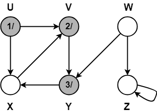
Step-03:


  • π[Y] = V
  • color[Y] = GREY
  • time = 2 + 1 = 3
  • d[Y] = 3


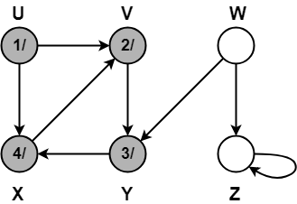
Step-04:


  • π[X] = Y
  • color[X] = GREY
  • time = 3 + 1 = 4
  • d[X] = 4


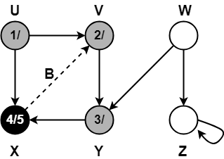
Step-05:


When DFS tries to extend the visit from vertex X to vertex V, it finds-

  • Vertex V is an ancestor of vertex X since it has already been discovered
  • Vertex V is GREY in color.


Thus, edge XV is a back edge.


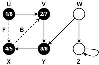
Step-06:


  • color[X] = BLACK
  • time = 4 + 1 = 5
  • f[X] = 5


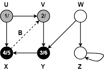
Step-07:


  • color[Y] = BLACK
  • time = 5 + 1 = 6
  • f[Y] = 6


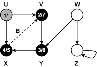
Step-08:


  • color[V] = BLACK
  • time = 6 + 1 = 7
  • f[V] = 7


Step-09:


When DFS tries to extend the visit from vertex U to vertex X, it finds-

  • Vertex X has already been completely processed i.e. vertex X has finished and is black.
  • But vertex U has still not finished.


Alternatively,

When DFS tries to extend the visit from vertex U to vertex X, it finds-

  • Color(X) = BLACK
  • d(X) > d(U)


Thus, edge UX is a forward edge.


Step-10:


  • color[U] = BLACK
  • time = 7 + 1 = 8
  • f[U] = 8


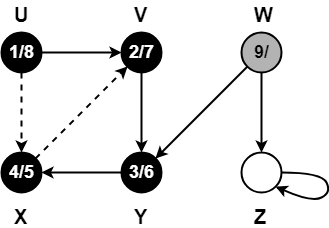
Step-11:


  • color[W] = GREY
  • time = 8 + 1 = 9
  • d[W] = 9


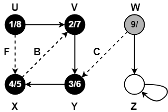
Step-12:


When DFS tries to extend the visit from vertex W to vertex Y, it finds-

  • Vertex Y has already been completely processed i.e. vertex Y has finished.
  • Vertex Y is neither a descendant nor an ancestor of vertex W.


Alternatively,

When DFS tries to extend the visit from vertex W to vertex Y, it finds-

  • Color(Y) = BLACK
  • d(Y) < d(W)


Thus, edge WY is a cross edge.


Step-13:


  • π[Z] = W
  • color[W] = GREY
  • time = 9 + 1 = 10
  • d[W] = 10


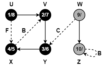
Step-14:


Since, self-loops are considered as back edges.

Therefore, self-loop present on vertex Z is considered as a back edge.


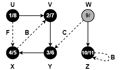
Step-15:


  • color[Z] = BLACK
  • time = 10 + 1 = 11
  • f[Z] = 11


Step-16:


  • color[W] = BLACK
  • time = 11 + 1 = 12
  • f[W] = 12


Since all the vertices have turned black, so we stop.

This is how a given graph is traversed using Depth First Search (DFS) technique.


To gain better understanding about Depth First Search Algorithm,

Watch this Video Lecture


Next Article- Breadth First Search


Get more notes and other study material of Design and Analysis of Algorithms.

Watch video lectures by visiting our YouTube channel LearnVidFun.
Master Theorem | Master Theorem Examples

Master Theorem-


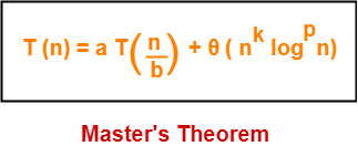
Master’s Theorem is a popular method for solving the recurrence relations.


Master’s theorem solves recurrence relations of the form-


Here, a >= 1, b > 1, k >= 0 and p is a real number.


Master Theorem Cases-


To solve recurrence relations using Master’s theorem, we compare a with bk.

Then, we follow the following cases-


Case-01:


If a > bk, then T(n) = θ (nlogba)


Case-02:


If a = band

  • If p < -1, then T(n) = θ (nlogba)
  • If p = -1, then T(n) = θ (nlogba.log2n)
  • If p > -1, then T(n) = θ (nlogba.logp+1n)


Case-03:


If a < band

  • If p < 0,  then T(n) = O (nk)
  • If p >= 0, then T(n) = θ (nklogpn)


PRACTICE PROBLEMS BASED ON MASTER THEOREM-


Problem-01:


Solve the following recurrence relation using Master’s theorem-

T(n) = 3T(n/2) + n2


Solution-


We compare the given recurrence relation with T(n) = aT(n/b) + θ (nklogpn).

Then, we have-

a = 3

b = 2

k = 2

p = 0


Now, a = 3 and bk = 22 = 4.

Clearly, a < bk.

So, we follow case-03.


Since p = 0, so we have-

T(n) = θ (nklogpn)

T(n) = θ (n2log0n)


Thus,

T(n) = θ (n2)


Problem-02:


Solve the following recurrence relation using Master’s theorem-

T(n) = 2T(n/2) + nlogn


Solution-


We compare the given recurrence relation with T(n) = aT(n/b) + θ (nklogpn).

Then, we have-

a = 2

b = 2

k = 1

p = 1


Now, a = 2 and bk = 21 = 2.

Clearly, a = bk.

So, we follow case-02.


Since p = 1, so we have-

T(n) = θ (nlogba.logp+1n)

T(n) = θ (nlog22.log1+1n)


Thus,

T(n) = θ (nlog2n)


Problem-03:


Solve the following recurrence relation using Master’s theorem-

T(n) = 2T(n/4) + n0.51


Solution-


We compare the given recurrence relation with T(n) = aT(n/b) + θ (nklogpn).

Then, we have-

a = 2

b = 4

k = 0.51

p = 0


Now, a = 2 and bk = 40.51 = 2.0279.

Clearly, a < bk.

So, we follow case-03.


Since p = 0, so we have-

T(n) = θ (nklogpn)

T(n) = θ (n0.51log0n)


Thus,

T(n) = θ (n0.51)


Problem-04:


Solve the following recurrence relation using Master’s theorem-

T(n) = √2T(n/2) + logn


Solution-


We compare the given recurrence relation with T(n) = aT(n/b) + θ (nklogpn).

Then, we have-

a = √2

b = 2

k = 0

p = 1


Now, a = √2 = 1.414 and bk = 20 = 1.

Clearly, a > bk.

So, we follow case-01.


So, we have-

T(n) = θ (nlogba)

T(n) = θ (nlog2√2)

T(n) = θ (n1/2)


Thus,

T(n) = θ (√n)


Problem-05:


Solve the following recurrence relation using Master’s theorem-

T(n) = 8T(n/4) – n2logn


Solution-


  • The given recurrence relation does not correspond to the general form of Master’s theorem.
  • So, it can not be solved using Master’s theorem.


Problem-06:


Solve the following recurrence relation using Master’s theorem-

T(n) = 3T(n/3) + n/2


Solution-


  • We write the given recurrence relation as T(n) = 3T(n/3) + n.
  • This is because in the general form, we have θ for function f(n) which hides constants in it.
  • Now, we can easily apply Master’s theorem.


We compare the given recurrence relation with T(n) = aT(n/b) + θ (nklogpn).

Then, we have-

a = 3

b = 3

k = 1

p = 0


Now, a = 3 and bk = 31 = 3.

Clearly, a = bk.

So, we follow case-02.


Since p = 0, so we have-

T(n) = θ (nlogba.logp+1n)

T(n) = θ (nlog33.log0+1n)

T(n) = θ (n1.log1n)


Thus,

T(n) = θ (nlogn)


Problem-07:


Form a recurrence relation for the following code and solve it using Master’s theorem-


A(n)
{
   if(n<=1)
     return 1;
   else
     return A(√n);
}


Solution-


  • We write a recurrence relation for the given code as T(n) = T(n) + 1.
  • Here 1 = Constant time taken for comparing and returning the value.
  • We can not directly apply Master’s Theorem on this recurrence relation.
  • This is because it does not correspond to the general form of Master’s theorem.
  • However, we can modify and bring it in the general form to apply Master’s theorem.


Let-

n = 2m    ……(1)

Then-

T(2m) = T(2m/2) + 1


Now, let T(2m) = S(m), then T(2m/2) = S(m/2)


So, we have-

S(m) = S(m/2) +1

Now, we can easily apply Master’s Theorem.


We compare the given recurrence relation with S(m) = aS(m/b) + θ (mklogpm).

Then, we have-

a = 1

b = 2

k = 0

p = 0


Now, a = 1 and bk = 20 = 1.

Clearly, a = bk.

So, we follow case-02.


Since p = 0, so we have-

S(m) = θ (mlogba.logp+1m)

S(m) = θ (mlog21.log0+1m)

S(m) = θ (m0.log1m)


Thus,

S(m) = θ(logm)    ……(2)


Now,

  • From (1), we have n = 2m.
  • So, logn = mlog2 which implies m = log2n.


Substituting in (2), we get-

S(m) = θ(loglog2n)

Or

T(n) = θ (loglog2n)


To gain better understanding about Master’s Theorem,

Watch this Video Lecture


Next Article- Recursion Tree


Get more notes and other study material of Design and Analysis of Algorithms.

Watch video lectures by visiting our YouTube channel LearnVidFun.
Separate Chaining Vs Open Addressing

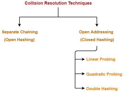
Collision Resolution Techniques-


In Hashing, collision resolution techniques are classified as-


  1. Separate Chaining
  2. Open Addressing


In this article, we will compare separate chaining and open addressing.


Separate Chaining Vs Open Addressing-


Separate Chaining

Open Addressing

Keys are stored inside the hash table as well as outside the hash table. All the keys are stored only inside the hash table.

No key is present outside the hash table.

The number of keys to be stored in the hash table can even exceed the size of the hash table. The number of keys to be stored in the hash table can never exceed the size of the hash table.
Deletion is easier. Deletion is difficult.
Extra space is required for the pointers to store the keys outside the hash table. No extra space is required.

Cache performance is poor.

This is because of linked lists which store the keys outside the hash table.

Cache performance is better.

This is because here no linked lists are used.

Some buckets of the hash table are never used which leads to wastage of space.

Buckets may be used even if no key maps to those particular buckets.


Which is the Preferred Technique?


The performance of both the techniques depend on the kind of operations that are required to be performed on the keys stored in the hash table-


Separate Chaining-


Separate Chaining is advantageous when it is required to perform all the following operations on the keys stored in the hash table-

  • Insertion Operation
  • Deletion Operation
  • Searching Operation


NOTE-


  • Deletion is easier in separate chaining.
  • This is because deleting a key from the hash table does not affect the other keys stored in the hash table.


Open Addressing-


Open addressing is advantageous when it is required to perform only the following operations on the keys stored in the hash table-

  • Insertion Operation
  • Searching Operation


NOTE-


  • Deletion is difficult in open addressing.
  • This is because deleting a key from the hash table requires some extra efforts.
  • After deleting a key, certain keys have to be rearranged.


To gain better understanding about Separate Chaining Vs Open Addressing,

Watch this Video Lecture


Get more notes and other study material of Data Structures.

Watch video lectures by visiting our YouTube channel LearnVidFun.