Data Structures and Algorithms | Gate Vidyalay

Selection Sort Algorithm | Example | Time Complexity

Design & Analysis of Algorithms

Selection Sort-

Selection sort is one of the easiest approaches to sorting.
It is inspired from the way in which we sort things out in day to day life.
It is an in-place sorting algorithm because it uses no auxiliary data structures while sorting.

How Selection Sort Works?

Consider the following elements are to be sorted in ascending order using selection sort-

6, 2, 11, 7, 5

Selection sort works as-

It finds the first smallest element (2).
It swaps it with the first element of the unordered list.
It finds the second smallest element (5).
It swaps it with the second element of the unordered list.
Similarly, it continues to sort the given elements.

As a result, sorted elements in ascending order are-

2, 5, 6, 7, 11

Selection Sort Algorithm-

Let A be an array with n elements. Then, selection sort algorithm used for sorting is as follows-

for (i = 0 ; i < n-1 ; i++)

{

   index = i;

   for(j = i+1 ; j < n ; j++)

   {

      if(A[j] < A[index])

      index = j;

   }

   temp = A[i];

   A[i] = A[index];

   A[index] = temp;

}

Here,

i = variable to traverse the array A
index = variable to store the index of minimum element
j = variable to traverse the unsorted sub-array
temp = temporary variable used for swapping

Selection Sort Example-

Consider the following elements are to be sorted in ascending order-

6, 2, 11, 7, 5

The above selection sort algorithm works as illustrated below-

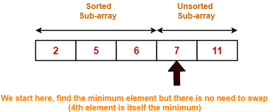
Step-01: For i = 0

Step-02: For i = 1

Step-03: For i = 2

Step-04: For i = 3

Step-05: For i = 4

Loop gets terminated as ‘i’ becomes 4.

The state of array after the loops are finished is as shown-

With each loop cycle,

The minimum element in unsorted sub-array is selected.
It is then placed at the correct location in the sorted sub-array until array A is completely sorted.

Time Complexity Analysis-

Selection sort algorithm consists of two nested loops.
Owing to the two nested loops, it has O(n²) time complexity.

	Time Complexity
Best Case	n²
Average Case	n²
Worst Case	n²

Space Complexity Analysis-

Selection sort is an in-place algorithm.
It performs all computation in the original array and no other array is used.
Hence, the space complexity works out to be O(1).

Important Notes-

Selection sort is not a very efficient algorithm when data sets are large.
This is indicated by the average and worst case complexities.
Selection sort uses minimum number of swap operations O(n) among all the sorting algorithms.

To gain better understanding about Selection Sort Algorithm,

Watch this Video Lecture

Next Article- Bubble Sort

Other Popular Sorting Algorithms-

Get more notes and other study material of Design and Analysis of Algorithms.

Watch video lectures by visiting our YouTube channel LearnVidFun.

AVL Tree Properties | Problems on AVL Tree

Data Structures

AVL Tree-

Before you go through this article, make sure that you have gone through the previous article on AVL Trees.

We have discussed-

AVL trees are self-balancing binary search trees.
In AVL trees, balancing factor of each node is either 0 or 1 or -1.

In this article, we will discuss AVL Tree Properties.

AVL Tree Properties-

Important properties of AVL tree are-

Property-01:

Maximum possible number of nodes in AVL tree of height H

= 2^H+1 – 1

Example-

Maximum possible number of nodes in AVL tree of height-3

= 2³⁺¹ – 1

= 16 – 1

= 15

Thus, in AVL tree of height-3, maximum number of nodes that can be inserted = 15.

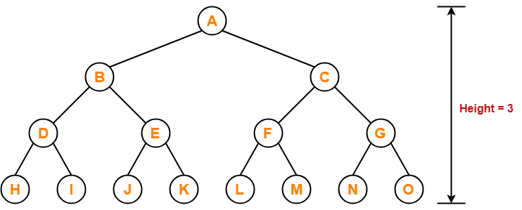
We can not insert more number of nodes in this AVL tree.

Property-02:

Minimum number of nodes in AVL Tree of height H is given by a recursive relation-

N(H) = N(H-1) + N(H-2) + 1

Base conditions for this recursive relation are-

N(0) = 1
N(1) = 2

Example-

Minimum possible number of nodes in AVL tree of height-3 = 7

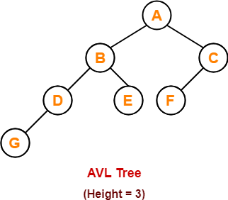
(For explanation, Refer problem-01)

Property-03:

Minimum possible height of AVL Tree using N nodes

= ⌊log₂N⌋

Example-

Minimum possible height of AVL Tree using 8 nodes

= ⌊log₂8⌋

= ⌊log₂2³⌋

= ⌊3log₂2⌋

= ⌊3⌋

= 3

Property-04:

Maximum height of AVL Tree using N nodes is calculated using recursive relation-

N(H) = N(H-1) + N(H-2) + 1

Base conditions for this recursive relation are-

N(0) = 1
N(1) = 2

NOTE-

If there are n nodes in AVL Tree, its maximum height can not exceed 1.44log₂n.
In other words, Worst case height of AVL Tree with n nodes = 1.44log₂n.

PRACTICE PROBLEMS BASED ON AVL TREE PROPERTIES-

Problem-01:

Find the minimum number of nodes required to construct AVL Tree of height = 3.

Solution-

We know, minimum number of nodes in AVL tree of height H is given by a recursive relation-

N(H) = N(H-1) + N(H-2) + 1

where N(0) = 1 and N(1) = 2

Step-01:

Substituting H = 3 in the recursive relation, we get-

N(3) = N(3-1) + N(3-2) + 1

N(3) = N(2) + N(1) + 1

N(3) = N(2) + 2 + 1 (Using base condition)

N(3) = N(2) + 3 …………(1)

To solve this recursive relation, we need the value of N(2).

Step-02:

Substituting H = 2 in the recursive relation, we get-

N(2) = N(2-1) + N(2-2) + 1

N(2) = N(1) + N(0) + 1

N(2) = 2 + 1 + 1 (Using base conditions)

∴ N(2) = 4 …………(2)

Step-03:

Using (2) in (1), we get-

N(3) = 4 + 3

∴ N(3) = 7

Thus, minimum number of nodes required to construct AVL tree of height-3 = 7.

Problem-02:

Find the minimum number of nodes required to construct AVL Tree of height = 4.

Solution-

We know, minimum number of nodes in AVL tree of height H is given by a recursive relation-

N(H) = N(H-1) + N(H-2) + 1

where N(0) = 1 and N(1) = 2

Step-01:

Substituting H = 4 in the recursive relation, we get-

N(4) = N(4-1) + N(4-2) + 1

N(4) = N(3) + N(2) + 1 …………(1)

To solve this recursive relation, we need the value of N(2) and N(3).

Step-02:

Substituting H = 2 in the recursive relation, we get-

N(2) = N(2-1) + N(2-2) + 1

N(2) = N(1) + N(0) + 1

N(2) = 2 + 1 + 1 (Using base conditions)

∴ N(2) = 4 …………(2)

Step-03:

Substituting H = 3 in the recursive relation, we get-

N(3) = N(3-1) + N(3-2) + 1

N(3) = N(2) + N(1) + 1

N(3) = 4 + 2 + 1 (Using (2) and base condition)

∴ N(3) = 7 …………(3)

Step-04:

Using (2) and (3) in (1), we get-

N(4) = 7 + 4 + 1

∴ N(4) = 12

Thus, minimum number of nodes required to construct AVL tree of height-4 = 12.

Problem-03:

What is the maximum height of any AVL tree with 10 nodes?

Solution-

For calculating the maximum height of AVL tree with n nodes, we use a recursive relation-

N(H) = N(H-1) + N(H-2) + 1

Step-01:

Substituting H = 2 in the recursive relation, we get-

N(2) = N(2-1) + N(2-2) + 1

N(2) = N(1) + N(0) + 1

N(2) = 2 + 1 + 1 (Using base conditions)

∴ N(2) = 4 …………(1)

So, minimum number of nodes required to construct AVL tree of height-2 = 4.

Step-02:

Substituting H = 3 in the recursive relation, we get-

N(3) = N(3-1) + N(3-2) + 1

N(3) = N(2) + N(1) + 1

N(3) = 4 + 2 + 1 (Using (1) and base condition)

∴ N(3) = 7 …………(2)

So, minimum number of nodes required to construct AVL tree of height-3 = 7.

Step-03:

Substituting H = 4 in the recursive relation, we get-

N(4) = N(4-1) + N(4-2) + 1

N(4) = N(3) + N(2) + 1

N(4) = 7 + 4 + 1 (Using (1) and (2))

∴ N(4) = 12

So, minimum number of nodes required to construct AVL tree of height-4 = 12.

But given number of nodes = 10 which is less than 12.

Thus, maximum height of AVL tree that can be obtained using 10 nodes = 3.

Problem-04:

What is the maximum height of any AVL tree with 77 nodes?

Solution-

For calculating the maximum height of AVL tree with n nodes, we use a recursive relation-

N(H) = N(H-1) + N(H-2) + 1

Step-01:

Substituting H = 2 in the recursive relation, we get-

N(2) = N(2-1) + N(2-2) + 1

N(2) = N(1) + N(0) + 1

N(2) = 2 + 1 + 1 (Using base conditions)

∴ N(2) = 4 …………(1)

So, minimum number of nodes required to construct AVL tree of height-2 = 4.

Step-02:

Substituting H = 3 in the recursive relation, we get-

N(3) = N(3-1) + N(3-2) + 1

N(3) = N(2) + N(1) + 1

N(3) = 4 + 2 + 1 (Using (1) and base condition)

∴ N(3) = 7 …………(2)

So, minimum number of nodes required to construct AVL tree of height-3 = 7.

Step-03:

Substituting H = 4 in the recursive relation, we get-

N(4) = N(4-1) + N(4-2) + 1

N(4) = N(3) + N(2) + 1

N(4) = 7 + 4 + 1 (Using (1) and (2))

∴ N(4) = 12 …………(3)

So, minimum number of nodes required to construct AVL tree of height-4 = 12.

Step-04:

Substituting H = 5 in the recursive relation, we get-

N(5) = N(5-1) + N(5-2) + 1

N(5) = N(4) + N(3) + 1

N(5) = 12 + 7 + 1 (Using (2) and (3))

∴ N(5) = 20 …………(4)

So, minimum number of nodes required to construct AVL tree of height-5 = 20.

Step-05:

Substituting H = 6 in the recursive relation, we get-

N(6) = N(6-1) + N(6-2) + 1

N(6) = N(5) + N(4) + 1

N(6) = 20 + 12 + 1 (Using (3) and (4))

∴ N(6) = 33 …………(5)

So, minimum number of nodes required to construct AVL tree of height-6 = 33.

Step-06:

Substituting H = 7 in the recursive relation, we get-

N(7) = N(7-1) + N(7-2) + 1

N(7) = N(6) + N(5) + 1

N(7) = 33 + 20 + 1 (Using (4) and (5))

∴ N(7) = 54 …………(6)

So, minimum number of nodes required to construct AVL tree of height-7 = 54.

Step-07:

Substituting H = 8 in the recursive relation, we get-

N(8) = N(8-1) + N(8-2) + 1

N(8) = N(7) + N(6) + 1

N(8) = 54 + 33 + 1 (Using (5) and (6))

∴ N(8) = 88 …………(6)

So, minimum number of nodes required to construct AVL tree of height-8 = 88.

But given number of nodes = 77 which is less than 88.

Thus, maximum height of AVL tree that can be obtained using 77 nodes = 7.

Next Article- Insertion in AVL Tree

Get more notes and other study material of Data Structures.

Watch video lectures by visiting our YouTube channel LearnVidFun.

AVL Tree Insertion | Insertion in AVL Tree

Data Structures

AVL Tree-

Before you go through this article, make sure that you have gone through the previous article on AVL Trees.

We have discussed-

AVL trees are self-balancing binary search trees.
In AVL trees, balancing factor of each node is either 0 or 1 or -1.

In this article, we will discuss insertion in AVL tree.

Insertion in AVL Tree-

Insertion Operation is performed to insert an element in the AVL Tree.

To insert an element in the AVL tree, follow the following steps-

Insert the element in the AVL tree in the same way the insertion is performed in BST.
After insertion, check the balance factor of each node of the resulting tree.

Now, following two cases are possible-

Case-01:

After the insertion, the balance factor of each node is either 0 or 1 or -1.
In this case, the tree is considered to be balanced.
Conclude the operation.
Insert the next element if any.

Case-02:

After the insertion, the balance factor of at least one node is not 0 or 1 or -1.
In this case, the tree is considered to be imbalanced.
Perform the suitable rotation to balance the tree.
After the tree is balanced, insert the next element if any.

Also Read- AVL Tree Properties

Rules To Remember-

Rule-01:

After inserting an element in the existing AVL tree,

Balance factor of only those nodes will be affected that lies on the path from the newly inserted node to the root node.

Rule-02:

To check whether the AVL tree is still balanced or not after the insertion,

There is no need to check the balance factor of every node.
Check the balance factor of only those nodes that lies on the path from the newly inserted node to the root node.

Rule-03:

After inserting an element in the AVL tree,

If tree becomes imbalanced, then there exists one particular node in the tree by balancing which the entire tree becomes balanced automatically.
To re balance the tree, balance that particular node.

To find that particular node,

Traverse the path from the newly inserted node to the root node.
Check the balance factor of each node that is encountered while traversing the path.
The first encountered imbalanced node will be the node that needs to be balanced.

To balance that node,

Count three nodes in the direction of leaf node.
Then, use the concept of AVL tree rotations to re balance the tree.

PRACTICE PROBLEM BASED ON AVL TREE INSERTION-

Problem-

Construct AVL Tree for the following sequence of numbers-

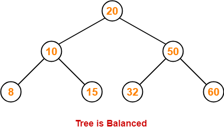
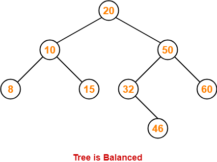
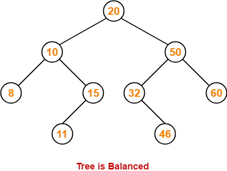
50 , 20 , 60 , 10 , 8 , 15 , 32 , 46 , 11 , 48

Solution-

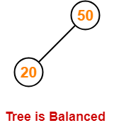
Step-01: Insert 50

Step-02: Insert 20

As 20 < 50, so insert 20 in 50’s left sub tree.

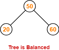
Step-03: Insert 60

As 60 > 50, so insert 60 in 50’s right sub tree.

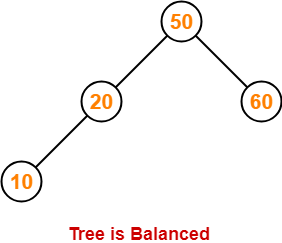
Step-04: Insert 10

As 10 < 50, so insert 10 in 50’s left sub tree.
As 10 < 20, so insert 10 in 20’s left sub tree.

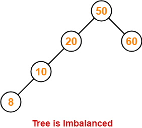
Step-05: Insert 8

As 8 < 50, so insert 8 in 50’s left sub tree.
As 8 < 20, so insert 8 in 20’s left sub tree.
As 8 < 10, so insert 8 in 10’s left sub tree.

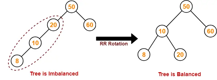
To balance the tree,

Find the first imbalanced node on the path from the newly inserted node (node 8) to the root node.
The first imbalanced node is node 20.
Now, count three nodes from node 20 in the direction of leaf node.
Then, use AVL tree rotation to balance the tree.

Following this, we have-

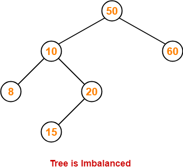
Step-06: Insert 15

As 15 < 50, so insert 15 in 50’s left sub tree.
As 15 > 10, so insert 15 in 10’s right sub tree.
As 15 < 20, so insert 15 in 20’s left sub tree.

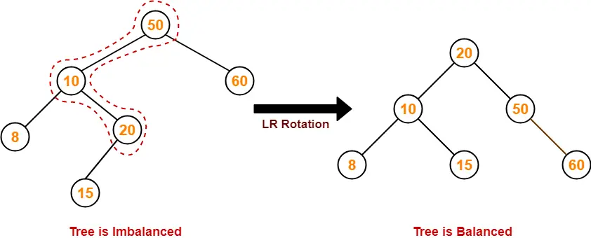
To balance the tree,

Find the first imbalanced node on the path from the newly inserted node (node 15) to the root node.
The first imbalanced node is node 50.
Now, count three nodes from node 50 in the direction of leaf node.
Then, use AVL tree rotation to balance the tree.

Following this, we have-

Step-07: Insert 32

As 32 > 20, so insert 32 in 20’s right sub tree.
As 32 < 50, so insert 32 in 50’s left sub tree.

Step-08: Insert 46

As 46 > 20, so insert 46 in 20’s right sub tree.
As 46 < 50, so insert 46 in 50’s left sub tree.
As 46 > 32, so insert 46 in 32’s right sub tree.

Step-09: Insert 11

As 11 < 20, so insert 11 in 20’s left sub tree.
As 11 > 10, so insert 11 in 10’s right sub tree.
As 11 < 15, so insert 11 in 15’s left sub tree.

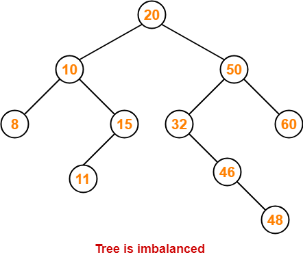
Step-10: Insert 48

As 48 > 20, so insert 48 in 20’s right sub tree.
As 48 < 50, so insert 48 in 50’s left sub tree.
As 48 > 32, so insert 48 in 32’s right sub tree.
As 48 > 46, so insert 48 in 46’s right sub tree.

To balance the tree,

Find the first imbalanced node on the path from the newly inserted node (node 48) to the root node.
The first imbalanced node is node 32.
Now, count three nodes from node 32 in the direction of leaf node.
Then, use AVL tree rotation to balance the tree.

Following this, we have-

This is the final balanced AVL tree after inserting all the given elements.

To gain better understanding of AVL Tree Insertion,

Watch this Video Lecture

Next Article- Heap Data Structure

Get more notes and other study material of Data Structures.

Watch video lectures by visiting our YouTube channel LearnVidFun.

Time Complexity of Binary Search Tree

Data Structures

Binary Search Tree-

Before you go through this article, make sure that you have gone through the previous article on BST Operations.

Commonly performed operations on binary search tree are-

Search Operation
Insertion Operation
Deletion Operation

In this article, we will discuss time complexity of BST Operations.

Time Complexity-

Time complexity of all BST Operations = O(h).
Here, h = Height of binary search tree

Now, let us discuss the worst case and best case.

Worst Case-

In worst case,

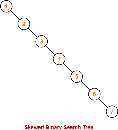
The binary search tree is a skewed binary search tree.
Height of the binary search tree becomes n.
So, Time complexity of BST Operations = O(n).

In this case, binary search tree is as good as unordered list with no benefits.

Best Case-

In best case,

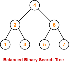
The binary search tree is a balanced binary search tree.
Height of the binary search tree becomes log(n).
So, Time complexity of BST Operations = O(logn).

To gain better understanding about Time Complexity of BST Operations,

Watch this Video Lecture

Download Handwritten Notes Here-

Next Article- Introduction to AVL Trees

Get more notes and other study material of Data Structures.

Watch video lectures by visiting our YouTube channel LearnVidFun.

AVL Tree | AVL Tree Example | AVL Tree Rotation

Data Structures

AVL Tree-

AVL trees are special kind of binary search trees.
In AVL trees, height of left subtree and right subtree of every node differs by at most one.
AVL trees are also called as self-balancing binary search trees.

Also Read- Binary Search Trees

Example-

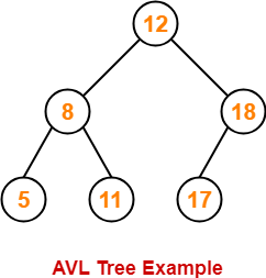
Following tree is an example of AVL tree-

This tree is an AVL tree because-

It is a binary search tree.
The difference between height of left subtree and right subtree of every node is at most one.

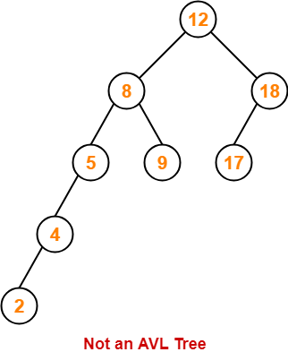
Following tree is not an example of AVL Tree-

This tree is not an AVL tree because-

The difference between height of left subtree and right subtree of root node = 4 – 2 = 2.
This difference is greater than one.

Balance Factor-

In AVL tree,

Balance factor is defined for every node.
Balance factor of a node = Height of its left subtree – Height of its right subtree

In AVL tree,

Balance factor of every node is either 0 or 1 or -1.

AVL Tree Operations-

Like BST Operations, commonly performed operations on AVL tree are-

Search Operation
Insertion Operation
Deletion Operation

Also Read- Insertion in AVL Tree

After performing any operation on AVL tree, the balance factor of each node is checked.

There are following two cases possible-

Case-01:

After the operation, the balance factor of each node is either 0 or 1 or -1.
In this case, the AVL tree is considered to be balanced.
The operation is concluded.

Case-02:

After the operation, the balance factor of at least one node is not 0 or 1 or -1.
In this case, the AVL tree is considered to be imbalanced.
Rotations are then performed to balance the tree.

AVL Tree Rotations-

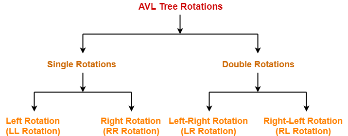
Rotation is the process of moving the nodes to make tree balanced.

Kinds of Rotations-

There are 4 kinds of rotations possible in AVL Trees-

Left Rotation (LL Rotation)
Right Rotation (RR Rotation)
Left-Right Rotation (LR Rotation)
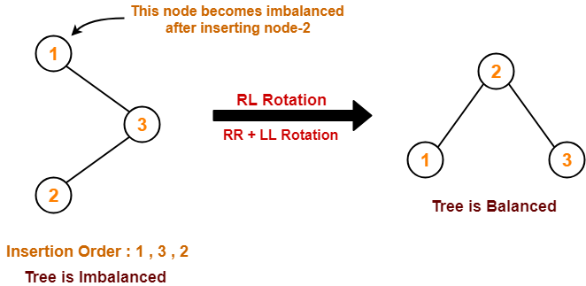
Right-Left Rotation (RL Rotation)

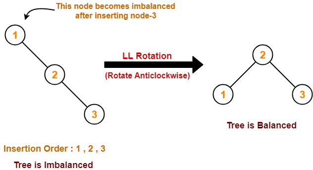
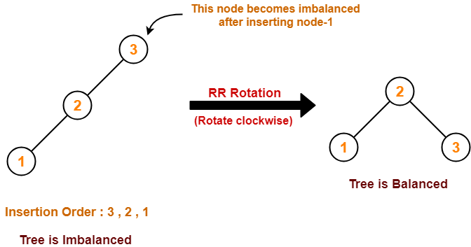
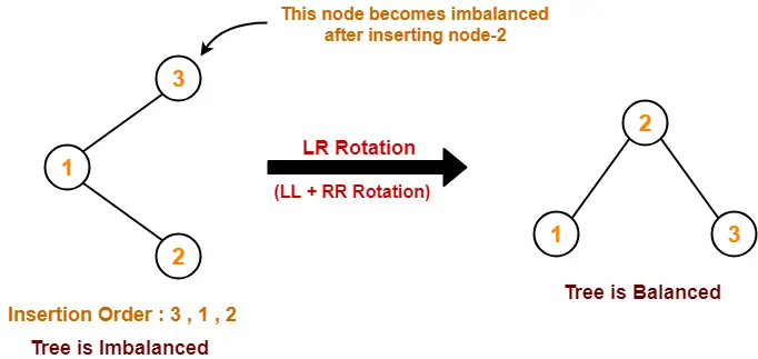
Cases Of Imbalance And Their Balancing Using Rotation Operations-

Case-01:

Case-02:

Case-03:

Case-04:

To gain better understanding about AVL Trees and Rotations,

Watch this Video Lecture

Download Handwritten Notes Here-

Next Article- AVL Tree Properties

Get more notes and other study material of Data Structures.

Watch video lectures by visiting our YouTube channel LearnVidFun.

Tag: Data Structures and Algorithms

Selection Sort-

How Selection Sort Works?

Selection Sort Algorithm-

Selection Sort Example-

Step-01: For i = 0

Step-02: For i = 1

Step-03: For i = 2

Step-04: For i = 3

Step-05: For i = 4

Time Complexity Analysis-

Space Complexity Analysis-

Important Notes-

Other Popular Sorting Algorithms-

AVL Tree-

AVL Tree Properties-

Property-01:

Example-

Property-02:

Example-

Property-03:

Example-

Property-04:

NOTE-

PRACTICE PROBLEMS BASED ON AVL TREE PROPERTIES-

Problem-01:

Solution-

Step-01:

Step-02:

Step-03:

Problem-02:

Solution-

Step-01:

Step-02:

Step-03:

Step-04:

Problem-03:

Solution-

Step-01:

Step-02:

Step-03:

Problem-04:

Solution-

Step-01:

Step-02:

Step-03:

Step-04:

Step-05:

Step-06:

Step-07:

AVL Tree-

Insertion in AVL Tree-

Case-01:

Case-02:

Rules To Remember-

Rule-01:

Rule-02:

Rule-03:

PRACTICE PROBLEM BASED ON AVL TREE INSERTION-

Problem-

Solution-

Step-01: Insert 50

Step-02: Insert 20

Step-03: Insert 60

Step-04: Insert 10

Step-05: Insert 8

Step-06: Insert 15

Step-07: Insert 32

Step-08: Insert 46

Step-09: Insert 11

Step-10: Insert 48

Binary Search Tree-

Time Complexity-

Worst Case-

Best Case-

Download Handwritten Notes Here-

AVL Tree-

Example-

Balance Factor-

AVL Tree Operations-