Tag: Data Structures and Algorithms For Beginners PDF

Depth First Search Algorithm | DFS Example

Depth First Search-


  • Depth First Search or DFS is a graph traversal algorithm.
  • It is used for traversing or searching a graph in a systematic fashion.
  • DFS uses a strategy that searches “deeper” in the graph whenever possible.
  • Stack data structure is used in the implementation of depth first search.


DFS Example-


Consider the following graph-
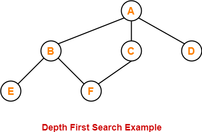


The depth first search traversal order of the above graph is-

A, B, E, F, C, D


Depth First Search Algorithm-


DFS (V,E)


for each vertex u in V[G]

do color[v] ← WHITE

π[v] ← NIL

time ← 0

for each vertex v in V[G]

do if color[v] ← WHITE

then Depth_First_Search(v)


Depth_First_Search (v)


color[v] ← GRAY

time ← time + 1

d[v] ← time

for each vertex u adjacent to v

do if color[u] ← WHITE

π[u] ← v

Depth_First_Search(u)

color[v] ← BLACK

time ← time + 1

f[v] ← time


Explanation-


The above depth first search algorithm is explained in the following steps-


Step-01


Create and maintain 4 variables for each vertex of the graph.

For any vertex ‘v’ of the graph, these 4 variables are-


1. color[v]-


  • This variable represents the color of the vertex ‘v’ at the given point of time.
  • The possible values of this variable are- WHITE, GREY and BLACK.
  • WHITE color of the vertex signifies that it has not been discovered yet.
  • GREY color of the vertex signifies that it has been discovered and it is being processed.
  • BLACK color of the vertex signifies that it has been completely processed.


2. Π[v]-


This variable represents the predecessor of vertex ‘v’.


3. d[v]-


This variable represents a timestamp when a vertex ‘v’ is discovered.


3. f[v]-


This variable represents a timestamp when the processing of vertex ‘v’ is completed.


Step-02


For each vertex of the graph, initialize the variables as-

  • color[v] = WHITE
  • π[v] = NIL
  • time = 0     (Global Variable acting as a timer)


Step-03


Repeat the following procedure until all the vertices of the graph become BLACK-

Consider any white vertex ‘v’ and call the following Depth_First_Search function on it.


Depth_First_Search (G,v)


1. color[v] = GRAY

2. time = time + 1

3. d[v] = time

4. For each adjacent WHITE vertex ‘u’ of ‘v’, set π[u] = v and call Depth_First_Search (G,u)

5. color[v] = BLACK

6. time = time + 1

7. f[v] = time


DFS Time Complexity-


The total running time for Depth First Search is θ (V+E).


Types of Edges in DFS-


After a DFS traversal of any graph G, all its edges can be put in one of the following 4 classes-


  1. Tree Edge
  2. Back Edge
  3. Forward Edge
  4. Cross Edge


1. Tree Edge-


  • A tree edge is an edge that is included in the DFS tree.


2. Back Edge-


An edge from a vertex ‘u’ to one of its ancestors ‘v’ is called as a back edge.

A self-loop is considered as a back edge.


A back edge is discovered when-

  • DFS tries to extend the visit from a vertex ‘u’ to vertex ‘v’
  • And vertex ‘v’ is found to be an ancestor of vertex ‘u’ and grey at that time.


3. Forward Edge-


An edge from a vertex ‘u’ to one of its descendants ‘v’ is called as a forward edge.


A forward edge is discovered when-

  • DFS tries to extend the visit from a vertex ‘u’ to a vertex ‘v’
  • And finds that color(v) = BLACK and d(v) > d(u).


4. Cross Edge-


An edge from a vertex ‘u’ to a vertex ‘v’ that is neither its ancestor nor its descendant is called as a cross edge.


A cross edge is discovered when-

  • DFS tries to extend the visit from a vertex ‘u’ to a vertex ‘v’
  • And finds that color(v) = BLACK and d(v) < d(u).


PRACTICE PROBLEM BASED ON DEPTH FIRST SEARCH-


Problem-


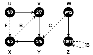
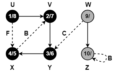
Compute the DFS tree for the graph given below-
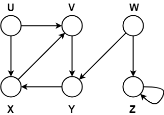


Also, show the discovery and finishing time for each vertex and classify the edges.


Solution-


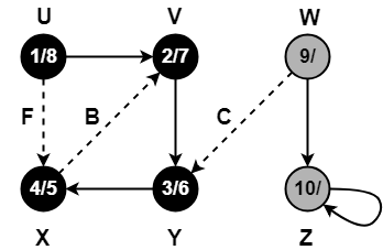
Initially for all the vertices of the graph, we set the variables as-

  • color[v] = WHITE
  • π[v] = NIL
  • time = 0 (Global)


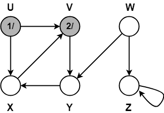
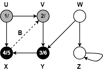
Let us start processing the graph from vertex U.


Step-01:


  • color[U] = GREY
  • time = 0 + 1 = 1
  • d[U] = 1


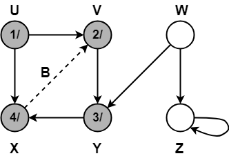
Step-02:


  • π[V] = U
  • color[V] = GREY
  • time = 1 + 1 = 2
  • d[V] = 2


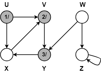
Step-03:


  • π[Y] = V
  • color[Y] = GREY
  • time = 2 + 1 = 3
  • d[Y] = 3


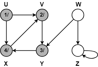
Step-04:


  • π[X] = Y
  • color[X] = GREY
  • time = 3 + 1 = 4
  • d[X] = 4


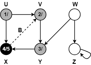
Step-05:


When DFS tries to extend the visit from vertex X to vertex V, it finds-

  • Vertex V is an ancestor of vertex X since it has already been discovered
  • Vertex V is GREY in color.


Thus, edge XV is a back edge.


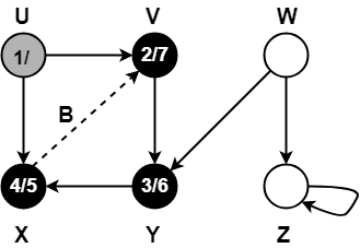
Step-06:


  • color[X] = BLACK
  • time = 4 + 1 = 5
  • f[X] = 5


Step-07:


  • color[Y] = BLACK
  • time = 5 + 1 = 6
  • f[Y] = 6


Step-08:


  • color[V] = BLACK
  • time = 6 + 1 = 7
  • f[V] = 7


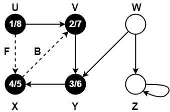
Step-09:


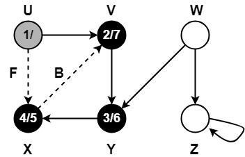
When DFS tries to extend the visit from vertex U to vertex X, it finds-

  • Vertex X has already been completely processed i.e. vertex X has finished and is black.
  • But vertex U has still not finished.


Alternatively,

When DFS tries to extend the visit from vertex U to vertex X, it finds-

  • Color(X) = BLACK
  • d(X) > d(U)


Thus, edge UX is a forward edge.


Step-10:


  • color[U] = BLACK
  • time = 7 + 1 = 8
  • f[U] = 8


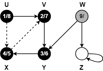
Step-11:


  • color[W] = GREY
  • time = 8 + 1 = 9
  • d[W] = 9


Step-12:


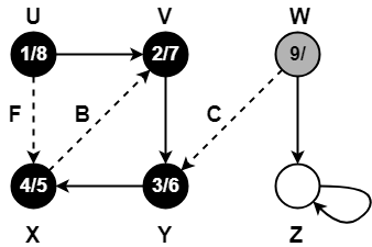
When DFS tries to extend the visit from vertex W to vertex Y, it finds-

  • Vertex Y has already been completely processed i.e. vertex Y has finished.
  • Vertex Y is neither a descendant nor an ancestor of vertex W.


Alternatively,

When DFS tries to extend the visit from vertex W to vertex Y, it finds-

  • Color(Y) = BLACK
  • d(Y) < d(W)


Thus, edge WY is a cross edge.


Step-13:


  • π[Z] = W
  • color[W] = GREY
  • time = 9 + 1 = 10
  • d[W] = 10


Step-14:


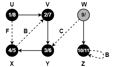
Since, self-loops are considered as back edges.

Therefore, self-loop present on vertex Z is considered as a back edge.


Step-15:


  • color[Z] = BLACK
  • time = 10 + 1 = 11
  • f[Z] = 11


Step-16:


  • color[W] = BLACK
  • time = 11 + 1 = 12
  • f[W] = 12


Since all the vertices have turned black, so we stop.

This is how a given graph is traversed using Depth First Search (DFS) technique.


To gain better understanding about Depth First Search Algorithm,

Watch this Video Lecture


Next Article- Breadth First Search


Get more notes and other study material of Design and Analysis of Algorithms.

Watch video lectures by visiting our YouTube channel LearnVidFun.
Master Theorem | Master Theorem Examples

Master Theorem-


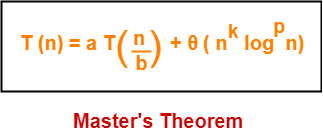
Master’s Theorem is a popular method for solving the recurrence relations.


Master’s theorem solves recurrence relations of the form-


Here, a >= 1, b > 1, k >= 0 and p is a real number.


Master Theorem Cases-


To solve recurrence relations using Master’s theorem, we compare a with bk.

Then, we follow the following cases-


Case-01:


If a > bk, then T(n) = θ (nlogba)


Case-02:


If a = band

  • If p < -1, then T(n) = θ (nlogba)
  • If p = -1, then T(n) = θ (nlogba.log2n)
  • If p > -1, then T(n) = θ (nlogba.logp+1n)


Case-03:


If a < band

  • If p < 0,  then T(n) = O (nk)
  • If p >= 0, then T(n) = θ (nklogpn)


PRACTICE PROBLEMS BASED ON MASTER THEOREM-


Problem-01:


Solve the following recurrence relation using Master’s theorem-

T(n) = 3T(n/2) + n2


Solution-


We compare the given recurrence relation with T(n) = aT(n/b) + θ (nklogpn).

Then, we have-

a = 3

b = 2

k = 2

p = 0


Now, a = 3 and bk = 22 = 4.

Clearly, a < bk.

So, we follow case-03.


Since p = 0, so we have-

T(n) = θ (nklogpn)

T(n) = θ (n2log0n)


Thus,

T(n) = θ (n2)


Problem-02:


Solve the following recurrence relation using Master’s theorem-

T(n) = 2T(n/2) + nlogn


Solution-


We compare the given recurrence relation with T(n) = aT(n/b) + θ (nklogpn).

Then, we have-

a = 2

b = 2

k = 1

p = 1


Now, a = 2 and bk = 21 = 2.

Clearly, a = bk.

So, we follow case-02.


Since p = 1, so we have-

T(n) = θ (nlogba.logp+1n)

T(n) = θ (nlog22.log1+1n)


Thus,

T(n) = θ (nlog2n)


Problem-03:


Solve the following recurrence relation using Master’s theorem-

T(n) = 2T(n/4) + n0.51


Solution-


We compare the given recurrence relation with T(n) = aT(n/b) + θ (nklogpn).

Then, we have-

a = 2

b = 4

k = 0.51

p = 0


Now, a = 2 and bk = 40.51 = 2.0279.

Clearly, a < bk.

So, we follow case-03.


Since p = 0, so we have-

T(n) = θ (nklogpn)

T(n) = θ (n0.51log0n)


Thus,

T(n) = θ (n0.51)


Problem-04:


Solve the following recurrence relation using Master’s theorem-

T(n) = √2T(n/2) + logn


Solution-


We compare the given recurrence relation with T(n) = aT(n/b) + θ (nklogpn).

Then, we have-

a = √2

b = 2

k = 0

p = 1


Now, a = √2 = 1.414 and bk = 20 = 1.

Clearly, a > bk.

So, we follow case-01.


So, we have-

T(n) = θ (nlogba)

T(n) = θ (nlog2√2)

T(n) = θ (n1/2)


Thus,

T(n) = θ (√n)


Problem-05:


Solve the following recurrence relation using Master’s theorem-

T(n) = 8T(n/4) – n2logn


Solution-


  • The given recurrence relation does not correspond to the general form of Master’s theorem.
  • So, it can not be solved using Master’s theorem.


Problem-06:


Solve the following recurrence relation using Master’s theorem-

T(n) = 3T(n/3) + n/2


Solution-


  • We write the given recurrence relation as T(n) = 3T(n/3) + n.
  • This is because in the general form, we have θ for function f(n) which hides constants in it.
  • Now, we can easily apply Master’s theorem.


We compare the given recurrence relation with T(n) = aT(n/b) + θ (nklogpn).

Then, we have-

a = 3

b = 3

k = 1

p = 0


Now, a = 3 and bk = 31 = 3.

Clearly, a = bk.

So, we follow case-02.


Since p = 0, so we have-

T(n) = θ (nlogba.logp+1n)

T(n) = θ (nlog33.log0+1n)

T(n) = θ (n1.log1n)


Thus,

T(n) = θ (nlogn)


Problem-07:


Form a recurrence relation for the following code and solve it using Master’s theorem-


A(n)
{
   if(n<=1)
     return 1;
   else
     return A(√n);
}


Solution-


  • We write a recurrence relation for the given code as T(n) = T(n) + 1.
  • Here 1 = Constant time taken for comparing and returning the value.
  • We can not directly apply Master’s Theorem on this recurrence relation.
  • This is because it does not correspond to the general form of Master’s theorem.
  • However, we can modify and bring it in the general form to apply Master’s theorem.


Let-

n = 2m    ……(1)

Then-

T(2m) = T(2m/2) + 1


Now, let T(2m) = S(m), then T(2m/2) = S(m/2)


So, we have-

S(m) = S(m/2) +1

Now, we can easily apply Master’s Theorem.


We compare the given recurrence relation with S(m) = aS(m/b) + θ (mklogpm).

Then, we have-

a = 1

b = 2

k = 0

p = 0


Now, a = 1 and bk = 20 = 1.

Clearly, a = bk.

So, we follow case-02.


Since p = 0, so we have-

S(m) = θ (mlogba.logp+1m)

S(m) = θ (mlog21.log0+1m)

S(m) = θ (m0.log1m)


Thus,

S(m) = θ(logm)    ……(2)


Now,

  • From (1), we have n = 2m.
  • So, logn = mlog2 which implies m = log2n.


Substituting in (2), we get-

S(m) = θ(loglog2n)

Or

T(n) = θ (loglog2n)


To gain better understanding about Master’s Theorem,

Watch this Video Lecture


Next Article- Recursion Tree


Get more notes and other study material of Design and Analysis of Algorithms.

Watch video lectures by visiting our YouTube channel LearnVidFun.

Job Sequencing With Deadlines | Algorithm | Example

Job Sequencing With Deadlines-


The sequencing of jobs on a single processor with deadline constraints is called as Job Sequencing with Deadlines.


Here-

  • You are given a set of jobs.
  • Each job has a defined deadline and some profit associated with it.
  • The profit of a job is given only when that job is completed within its deadline.
  • Only one processor is available for processing all the jobs.
  • Processor takes one unit of time to complete a job.


The problem states-

“How can the total profit be maximized if only one job can be completed at a time?”


Approach to Solution-


  • A feasible solution would be a subset of jobs where each job of the subset gets completed within its deadline.
  • Value of the feasible solution would be the sum of profit of all the jobs contained in the subset.
  • An optimal solution of the problem would be a feasible solution which gives the maximum profit.


Greedy Algorithm-


Greedy Algorithm is adopted to determine how the next job is selected for an optimal solution.

The greedy algorithm described below always gives an optimal solution to the job sequencing problem-


Step-01:


  • Sort all the given jobs in decreasing order of their profit.


Step-02:


  • Check the value of maximum deadline.
  • Draw a Gantt chart where maximum time on Gantt chart is the value of maximum deadline.


Step-03:


  • Pick up the jobs one by one.
  • Put the job on Gantt chart as far as possible from 0 ensuring that the job gets completed before its deadline.


PRACTICE PROBLEM BASED ON JOB SEQUENCING WITH DEADLINES-


Problem-


Given the jobs, their deadlines and associated profits as shown-


Jobs J1 J2 J3 J4 J5 J6
Deadlines 5 3 3 2 4 2
Profits 200 180 190 300 120 100


Answer the following questions-

  1. Write the optimal schedule that gives maximum profit.
  2. Are all the jobs completed in the optimal schedule?
  3. What is the maximum earned profit?


Solution-


Step-01:


Sort all the given jobs in decreasing order of their profit-


Jobs J4 J1 J3 J2 J5 J6
Deadlines 2 5 3 3 4 2
Profits 300 200 190 180 120 100


Step-02:


Value of maximum deadline = 5.

So, draw a Gantt chart with maximum time on Gantt chart = 5 units as shown-


Now,

  • We take each job one by one in the order they appear in Step-01.
  • We place the job on Gantt chart as far as possible from 0.


Step-03:


  • We take job J4.
  • Since its deadline is 2, so we place it in the first empty cell before deadline 2 as-


Step-04:


  • We take job J1.
  • Since its deadline is 5, so we place it in the first empty cell before deadline 5 as-


Step-05:


  • We take job J3.
  • Since its deadline is 3, so we place it in the first empty cell before deadline 3 as-


Step-06:


  • We take job J2.
  • Since its deadline is 3, so we place it in the first empty cell before deadline 3.
  • Since the second and third cells are already filled, so we place job J2 in the first cell as-


Step-07:


  • Now, we take job J5.
  • Since its deadline is 4, so we place it in the first empty cell before deadline 4 as-


Now,

  • The only job left is job J6 whose deadline is 2.
  • All the slots before deadline 2 are already occupied.
  • Thus, job J6 can not be completed.


Now, the given questions may be answered as-


Part-01:


The optimal schedule is-

J2  , J4 , J3 , J5 , J1

This is the required order in which the jobs must be completed in order to obtain the maximum profit.


Part-02:


  • All the jobs are not completed in optimal schedule.
  • This is because job J6 could not be completed within its deadline.


Part-03:


Maximum earned profit

= Sum of profit of all the jobs in optimal schedule

= Profit of job J2 + Profit of job J4 + Profit of job J3 + Profit of job J5 + Profit of job J1

= 180 + 300 + 190 + 120 + 200

= 990 units


To gain better understanding about Job Sequencing With Deadlines,

Watch this Video Lecture


Next Article- Huffman Coding


Get more notes and other study material of Design and Analysis of Algorithms.

Watch video lectures by visiting our YouTube channel LearnVidFun.

Travelling Salesman Problem | Branch & Bound

Travelling Salesman Problem-


You are given-

  • A set of some cities
  • Distance between every pair of cities


Travelling Salesman Problem states-

  • A salesman has to visit every city exactly once.
  • He has to come back to the city from where he starts his journey.
  • What is the shortest possible route that the salesman must follow to complete his tour?


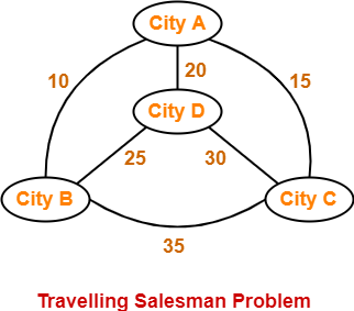
Example-


The following graph shows a set of cities and distance between every pair of cities-


If salesman starting city is A, then a TSP tour in the graph is-

A → B → D → C → A


Cost of the tour

= 10 + 25 + 30 + 15

= 80 units


In this article, we will discuss how to solve travelling salesman problem using branch and bound approach with example.


PRACTICE PROBLEM BASED ON TRAVELLING SALESMAN PROBLEM USING BRANCH AND BOUND APPROACH-


Problem-


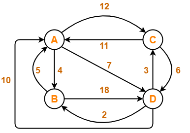
Solve Travelling Salesman Problem using Branch and Bound Algorithm in the following graph-


Solution-


Step-01:


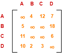
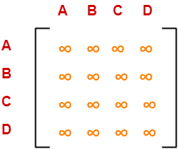
Write the initial cost matrix and reduce it-


Rules

  • To reduce a matrix, perform the row reduction and column reduction of the matrix separately.
  • A row or a column is said to be reduced if it contains at least one entry ‘0’ in it.


Row Reduction-


Consider the rows of above matrix one by one.


If the row already contains an entry ‘0’, then-

  • There is no need to reduce that row.


If the row does not contains an entry ‘0’, then-

  • Reduce that particular row.
  • Select the least value element from that row.
  • Subtract that element from each element of that row.
  • This will create an entry ‘0’ in that row, thus reducing that row.


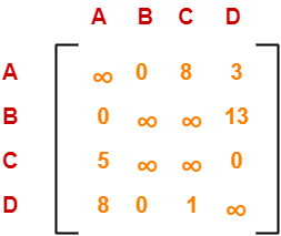
Following this, we have-

  • Reduce the elements of row-1 by 4.
  • Reduce the elements of row-2 by 5.
  • Reduce the elements of row-3 by 6.
  • Reduce the elements of row-4 by 2.


Performing this, we obtain the following row-reduced matrix-


Column Reduction-


Consider the columns of above row-reduced matrix one by one.


If the column already contains an entry ‘0’, then-

  • There is no need to reduce that column.


If the column does not contains an entry ‘0’, then-

  • Reduce that particular column.
  • Select the least value element from that column.
  • Subtract that element from each element of that column.
  • This will create an entry ‘0’ in that column, thus reducing that column.


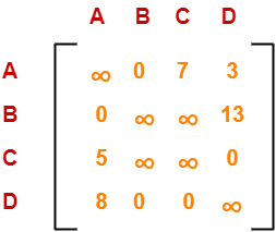
Following this, we have-

  • There is no need to reduce column-1.
  • There is no need to reduce column-2.
  • Reduce the elements of column-3 by 1.
  • There is no need to reduce column-4.


Performing this, we obtain the following column-reduced matrix-


Finally, the initial distance matrix is completely reduced.

Now, we calculate the cost of node-1 by adding all the reduction elements.


Cost(1)

= Sum of all reduction elements

= 4 + 5 + 6 + 2 + 1

= 18


Step-02:


  • We consider all other vertices one by one.
  • We select the best vertex where we can land upon to minimize the tour cost.


Choosing To Go To Vertex-B: Node-2 (Path A → B)


  • From the reduced matrix of step-01, M[A,B] = 0
  • Set row-A and column-B to 
  • Set M[B,A] = 


Now, resulting cost matrix is-


Now,

  • We reduce this matrix.
  • Then, we find out the cost of node-02.


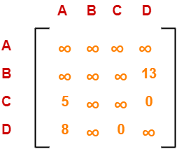
Row Reduction-


  • We can not reduce row-1 as all its elements are ∞.
  • Reduce all the elements of row-2 by 13.
  • There is no need to reduce row-3.
  • There is no need to reduce row-4.


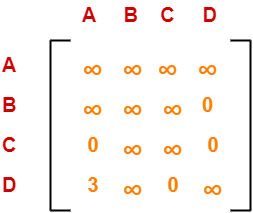
Performing this, we obtain the following row-reduced matrix-


Column Reduction-


  • Reduce the elements of column-1 by 5.
  • We can not reduce column-2 as all its elements are ∞.
  • There is no need to reduce column-3.
  • There is no need to reduce column-4.


Performing this, we obtain the following column-reduced matrix-


Finally, the matrix is completely reduced.

Now, we calculate the cost of node-2.


Cost(2)

= Cost(1) + Sum of reduction elements + M[A,B]

= 18 + (13 + 5) + 0

= 36


Choosing To Go To Vertex-C: Node-3 (Path A → C)


  • From the reduced matrix of step-01, M[A,C] = 7
  • Set row-A and column-C to 
  • Set M[C,A] = 


Now, resulting cost matrix is-


Now,

  • We reduce this matrix.
  • Then, we find out the cost of node-03.


Row Reduction-


  • We can not reduce row-1 as all its elements are ∞.
  • There is no need to reduce row-2.
  • There is no need to reduce row-3.
  • There is no need to reduce row-4.


Thus, the matrix is already row-reduced.


Column Reduction-


  • There is no need to reduce column-1.
  • There is no need to reduce column-2.
  • We can not reduce column-3 as all its elements are ∞.
  • There is no need to reduce column-4.


Thus, the matrix is already column reduced.

Finally, the matrix is completely reduced.

Now, we calculate the cost of node-3.


Cost(3)

= Cost(1) + Sum of reduction elements + M[A,C]

= 18 + 0 + 7

= 25


Choosing To Go To Vertex-D: Node-4 (Path A → D)


  • From the reduced matrix of step-01, M[A,D] = 3
  • Set row-A and column-D to 
  • Set M[D,A] = 


Now, resulting cost matrix is-


Now,

  • We reduce this matrix.
  • Then, we find out the cost of node-04.


Row Reduction-


  • We can not reduce row-1 as all its elements are ∞.
  • There is no need to reduce row-2.
  • Reduce all the elements of row-3 by 5.
  • There is no need to reduce row-4.


Performing this, we obtain the following row-reduced matrix-


Column Reduction-


  • There is no need to reduce column-1.
  • There is no need to reduce column-2.
  • There is no need to reduce column-3.
  • We can not reduce column-4 as all its elements are ∞.


Thus, the matrix is already column-reduced.

Finally, the matrix is completely reduced.

Now, we calculate the cost of node-4.


Cost(4)

= Cost(1) + Sum of reduction elements + M[A,D]

= 18 + 5 + 3

= 26


Thus, we have-

  • Cost(2) = 36 (for Path A → B)
  • Cost(3) = 25 (for Path A → C)
  • Cost(4) = 26 (for Path A → D)


We choose the node with the lowest cost.

Since cost for node-3 is lowest, so we prefer to visit node-3.

Thus, we choose node-3 i.e. path A → C.


Step-03:


We explore the vertices B and D from node-3.

We now start from the cost matrix at node-3 which is-


Cost(3) = 25


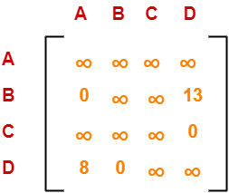
Choosing To Go To Vertex-B: Node-5 (Path A → C → B)


  • From the reduced matrix of step-02, M[C,B] = 
  • Set row-C and column-B to 
  • Set M[B,A] = 


Now, resulting cost matrix is-


Now,

  • We reduce this matrix.
  • Then, we find out the cost of node-5.


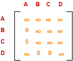
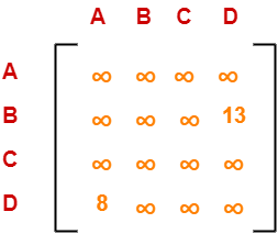
Row Reduction-


  • We can not reduce row-1 as all its elements are ∞.
  • Reduce all the elements of row-2 by 13.
  • We can not reduce row-3 as all its elements are ∞.
  • Reduce all the elements of row-4 by 8.


Performing this, we obtain the following row-reduced matrix-


Column Reduction-


  • There is no need to reduce column-1.
  • We can not reduce column-2 as all its elements are ∞.
  • We can not reduce column-3 as all its elements are ∞.
  • There is no need to reduce column-4.


Thus, the matrix is already column reduced.

Finally, the matrix is completely reduced.

Now, we calculate the cost of node-5.


Cost(5)

= cost(3) + Sum of reduction elements + M[C,B]

= 25 + (13 + 8) +

=


Choosing To Go To Vertex-D: Node-6 (Path A → C → D)


  • From the reduced matrix of step-02, M[C,D] = 
  • Set row-C and column-D to 
  • Set M[D,A] = 


Now, resulting cost matrix is-


Now,

  • We reduce this matrix.
  • Then, we find out the cost of node-6.


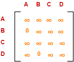
Row Reduction-


  • We can not reduce row-1 as all its elements are ∞.
  • There is no need to reduce row-2.
  • We can not reduce row-3 as all its elements are ∞.
  • We can not reduce row-4 as all its elements are ∞.


Thus, the matrix is already row reduced.


Column Reduction-


  • There is no need to reduce column-1.
  • We can not reduce column-2 as all its elements are ∞.
  • We can not reduce column-3 as all its elements are ∞.
  • We can not reduce column-4 as all its elements are ∞.


Thus, the matrix is already column reduced.

Finally, the matrix is completely reduced.

Now, we calculate the cost of node-6.


Cost(6)

= cost(3) + Sum of reduction elements + M[C,D]

= 25 + 0 + 0

= 25


Thus, we have-

  • Cost(5) =  (for Path A → C → B)
  • Cost(6) = 25 (for Path A → C → D)


We choose the node with the lowest cost.

Since cost for node-6 is lowest, so we prefer to visit node-6.

Thus, we choose node-6 i.e. path C → D.


Step-04:


We explore vertex B from node-6.

We start with the cost matrix at node-6 which is-


Cost(6) = 25


Choosing To Go To Vertex-B: Node-7 (Path A → C → D → B)


  • From the reduced matrix of step-03, M[D,B] = 0
  • Set row-D and column-B to 
  • Set M[B,A] = 


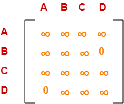
Now, resulting cost matrix is-


Now,

  • We reduce this matrix.
  • Then, we find out the cost of node-7.


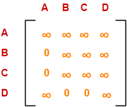
Row Reduction-


  • We can not reduce row-1 as all its elements are ∞.
  • We can not reduce row-2 as all its elements are ∞.
  • We can not reduce row-3 as all its elements are ∞.
  • We can not reduce row-4 as all its elements are ∞.


Column Reduction-


  • We can not reduce column-1 as all its elements are ∞.
  • We can not reduce column-2 as all its elements are ∞.
  • We can not reduce column-3 as all its elements are ∞.
  • We can not reduce column-4 as all its elements are ∞.


Thus, the matrix is already column reduced.

Finally, the matrix is completely reduced.

All the entries have become ∞.

Now, we calculate the cost of node-7.


Cost(7)

= cost(6) + Sum of reduction elements + M[D,B]

= 25 + 0 + 0

= 25


Thus,

  • Optimal path is: A → C → D → B → A
  • Cost of Optimal path = 25 units


To gain better understanding about Travelling Salesman Problem,

Watch this Video Lecture


Get more notes and other study material of Design and Analysis of Algorithms.

Watch video lectures by visiting our YouTube channel LearnVidFun.

Dijkstra Algorithm | Example | Time Complexity

Dijkstra Algorithm-


  • Dijkstra Algorithm is a very famous greedy algorithm.
  • It is used for solving the single source shortest path problem.
  • It computes the shortest path from one particular source node to all other remaining nodes of the graph.


Also Read- Shortest Path Problem


Conditions-


It is important to note the following points regarding Dijkstra Algorithm-

  • Dijkstra algorithm works only for connected graphs.
  • Dijkstra algorithm works only for those graphs that do not contain any negative weight edge.
  • The actual Dijkstra algorithm does not output the shortest paths.
  • It only provides the value or cost of the shortest paths.
  • By making minor modifications in the actual algorithm, the shortest paths can be easily obtained.
  • Dijkstra algorithm works for directed as well as undirected graphs.


Dijkstra Algorithm-


dist[S] ← 0                                                  // The distance to source vertex is set to 0

Π[S] ← NIL                                                   // The predecessor of source vertex is set as NIL

for all v ∈ V - {S}                                          // For all other vertices

        do dist[v] ← ∞                                       // All other distances are set to ∞

        Π[v] ← NIL                                           // The predecessor of all other vertices is set as NIL

S ← ∅                                                        // The set of vertices that have been visited 'S' is initially empty

Q ← V                                                        // The queue 'Q' initially contains all the vertices

while Q ≠ ∅                                                  // While loop executes till the queue is not empty

        do u ← mindistance (Q, dist)                         // A vertex from Q with the least distance is selected

        S ← S ∪ {u}                                          // Vertex 'u' is added to 'S' list of vertices that have been visited

for all v ∈ neighbors[u]                                     // For all the neighboring vertices of vertex 'u'

        do if dist[v] > dist[u] + w(u,v)                     // if any new shortest path is discovered

                then dist[v] ← dist[u] + w(u,v)              // The new value of the shortest path is selected

return dist


Implementation-


The implementation of above Dijkstra Algorithm is explained in the following steps-


Step-01:


In the first step. two sets are defined-

  • One set contains all those vertices which have been included in the shortest path tree.
  • In the beginning, this set is empty.
  • Other set contains all those vertices which are still left to be included in the shortest path tree.
  • In the beginning, this set contains all the vertices of the given graph.


Step-02:


For each vertex of the given graph, two variables are defined as-

  • Π[v] which denotes the predecessor of vertex ‘v’
  • d[v] which denotes the shortest path estimate of vertex ‘v’ from the source vertex.


Initially, the value of these variables is set as-

  • The value of variable ‘Π’ for each vertex is set to NIL i.e. Π[v] = NIL
  • The value of variable ‘d’ for source vertex is set to 0 i.e. d[S] = 0
  • The value of variable ‘d’ for remaining vertices is set to ∞ i.e. d[v] = ∞


Step-03:


The following procedure is repeated until all the vertices of the graph are processed-

  • Among unprocessed  vertices, a vertex with minimum value of variable ‘d’ is chosen.
  • Its outgoing edges are relaxed.
  • After relaxing the edges for that vertex, the sets created in step-01 are updated.


What is Edge Relaxation?


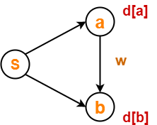
Consider the edge (a,b) in the following graph-


Here, d[a] and d[b] denotes the shortest path estimate for vertices a and b respectively from the source vertex ‘S’.

Now,

If d[a] + w < d[b]

then d[b] = d[a] + w and Π[b] = a

This is called as edge relaxation.


Time Complexity Analysis-


Case-01:


This case is valid when-

  • The given graph G is represented as an adjacency matrix.
  • Priority queue Q is represented as an unordered list.


Here,

  • A[i,j] stores the information about edge (i,j).
  • Time taken for selecting i with the smallest dist is O(V).
  • For each neighbor of i, time taken for updating dist[j] is O(1) and there will be maximum V neighbors.
  • Time taken for each iteration of the loop is O(V) and one vertex is deleted from Q.
  • Thus, total time complexity becomes O(V2).


Case-02:


This case is valid when-

  • The given graph G is represented as an adjacency list.
  • Priority queue Q is represented as a binary heap.


Here,

  • With adjacency list representation, all vertices of the graph can be traversed using BFS in O(V+E) time.
  • In min heap, operations like extract-min and decrease-key value takes O(logV) time.
  • So, overall time complexity becomes O(E+V) x O(logV) which is O((E + V) x logV) = O(ElogV)
  • This time complexity can be reduced to O(E+VlogV) using Fibonacci heap.


PRACTICE PROBLEM BASED ON DIJKSTRA ALGORITHM-


Problem-


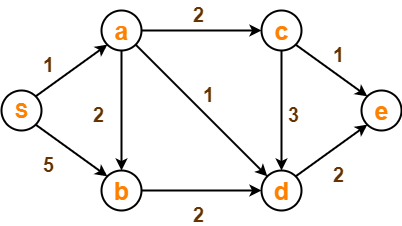
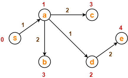
Using Dijkstra’s Algorithm, find the shortest distance from source vertex ‘S’ to remaining vertices in the following graph-


Also, write the order in which the vertices are visited.


Solution-


Step-01:


The following two sets are created-

  • Unvisited set : {S , a , b , c , d , e}
  • Visited set     : { }


Step-02:


The two variables  Π and d are created for each vertex and initialized as-

  • Π[S] = Π[a] = Π[b] = Π[c] = Π[d] = Π[e] = NIL
  • d[S] = 0
  • d[a] = d[b] = d[c] = d[d] = d[e] = ∞


Step-03:


  • Vertex ‘S’ is chosen.
  • This is because shortest path estimate for vertex ‘S’ is least.
  • The outgoing edges of vertex ‘S’ are relaxed.


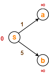
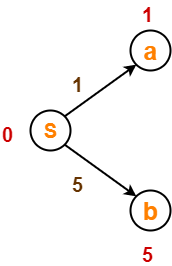
Before Edge Relaxation-


Now,

  • d[S] + 1 = 0 + 1 = 1 < ∞

∴ d[a] = 1 and Π[a] = S

  • d[S] + 5 = 0 + 5 = 5 < ∞

∴ d[b] = 5 and Π[b] = S


After edge relaxation, our shortest path tree is-


Now, the sets are updated as-

  • Unvisited set : {a , b , c , d , e}
  • Visited set : {S}


Step-04:


  • Vertex ‘a’ is chosen.
  • This is because shortest path estimate for vertex ‘a’ is least.
  • The outgoing edges of vertex ‘a’ are relaxed.


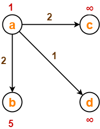
Before Edge Relaxation-


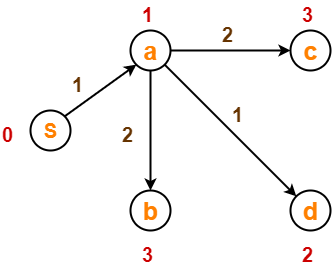
Now,

  • d[a] + 2 = 1 + 2 = 3 < ∞

∴ d[c] = 3 and Π[c] = a

  • d[a] + 1 = 1 + 1 = 2 < ∞

∴ d[d] = 2 and Π[d] = a

  • d[b] + 2 = 1 + 2 = 3 < 5

∴ d[b] = 3 and Π[b] = a


After edge relaxation, our shortest path tree is-


Now, the sets are updated as-

  • Unvisited set : {b , c , d , e}
  • Visited set : {S , a}


Step-05:


  • Vertex ‘d’ is chosen.
  • This is because shortest path estimate for vertex ‘d’ is least.
  • The outgoing edges of vertex ‘d’ are relaxed.


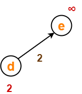
Before Edge Relaxation-


Now,

  • d[d] + 2 = 2 + 2 = 4 < ∞

∴ d[e] = 4 and Π[e] = d


After edge relaxation, our shortest path tree is-


Now, the sets are updated as-

  • Unvisited set : {b , c , e}
  • Visited set : {S , a , d}


Step-06:


  • Vertex ‘b’ is chosen.
  • This is because shortest path estimate for vertex ‘b’ is least.
  • Vertex ‘c’ may also be chosen since for both the vertices, shortest path estimate is least.
  • The outgoing edges of vertex ‘b’ are relaxed.


Before Edge Relaxation-


Now,

  • d[b] + 2 = 3 + 2 = 5 > 2

∴ No change


After edge relaxation, our shortest path tree remains the same as in Step-05.

Now, the sets are updated as-

  • Unvisited set : {c , e}
  • Visited set     : {S , a , d , b}


Step-07:


  • Vertex ‘c’ is chosen.
  • This is because shortest path estimate for vertex ‘c’ is least.
  • The outgoing edges of vertex ‘c’ are relaxed.


Before Edge Relaxation-


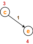
Now,

  • d[c] + 1 = 3 + 1 = 4 = 4

∴ No change


After edge relaxation, our shortest path tree remains the same as in Step-05.

Now, the sets are updated as-

  • Unvisited set : {e}
  • Visited set : {S , a , d , b , c}


Step-08:


  • Vertex ‘e’ is chosen.
  • This is because shortest path estimate for vertex ‘e’ is least.
  • The outgoing edges of vertex ‘e’ are relaxed.
  • There are no outgoing edges for vertex ‘e’.
  • So, our shortest path tree remains the same as in Step-05.


Now, the sets are updated as-

  • Unvisited set : { }
  • Visited set : {S , a , d , b , c , e}


Now,

  • All vertices of the graph are processed.
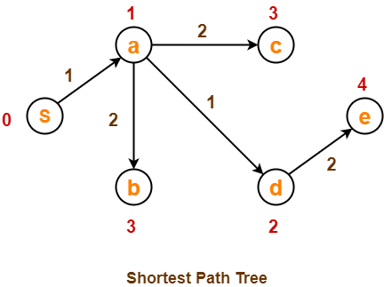
  • Our final shortest path tree is as shown below.
  • It represents the shortest path from source vertex ‘S’ to all other remaining vertices.


The order in which all the vertices are processed is :

S , a , d , b , c , e.


To gain better understanding about Dijkstra Algorithm,

Watch this Video Lecture


Next Article- Floyd-Warshall Algorithm


Get more notes and other study material of Design and Analysis of Algorithms.

Watch video lectures by visiting our YouTube channel LearnVidFun.