Knapsack Problem-
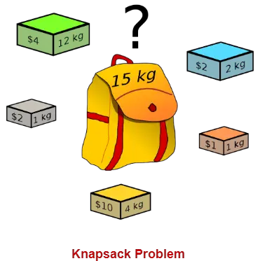
You are given the following-
- A knapsack (kind of shoulder bag) with limited weight capacity.
- Few items each having some weight and value.
The problem states-
Which items should be placed into the knapsack such that-
- The value or profit obtained by putting the items into the knapsack is maximum.
- And the weight limit of the knapsack does not exceed.

Knapsack Problem Variants-
Knapsack problem has the following two variants-
- Fractional Knapsack Problem
- 0/1 Knapsack Problem
In this article, we will discuss about 0/1 Knapsack Problem.
0/1 Knapsack Problem-
In 0/1 Knapsack Problem,
- As the name suggests, items are indivisible here.
- We can not take the fraction of any item.
- We have to either take an item completely or leave it completely.
- It is solved using dynamic programming approach.
Also Read- Fractional Knapsack Problem
0/1 Knapsack Problem Using Dynamic Programming-
Consider-
- Knapsack weight capacity = w
- Number of items each having some weight and value = n
0/1 knapsack problem is solved using dynamic programming in the following steps-
Step-01:
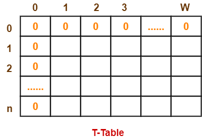
- Draw a table say ‘T’ with (n+1) number of rows and (w+1) number of columns.
- Fill all the boxes of 0th row and 0th column with zeroes as shown-

Step-02:
Start filling the table row wise top to bottom from left to right.
Use the following formula-
T (i , j) = max { T ( i-1 , j ) , valuei + T( i-1 , j – weighti ) }
Here, T(i , j) = maximum value of the selected items if we can take items 1 to i and have weight restrictions of j.
- This step leads to completely filling the table.
- Then, value of the last box represents the maximum possible value that can be put into the knapsack.
Step-03:
To identify the items that must be put into the knapsack to obtain that maximum profit,
- Consider the last column of the table.
- Start scanning the entries from bottom to top.
- On encountering an entry whose value is not same as the value stored in the entry immediately above it, mark the row label of that entry.
- After all the entries are scanned, the marked labels represent the items that must be put into the knapsack.
Time Complexity-
- Each entry of the table requires constant time θ(1) for its computation.
- It takes θ(nw) time to fill (n+1)(w+1) table entries.
- It takes θ(n) time for tracing the solution since tracing process traces the n rows.
- Thus, overall θ(nw) time is taken to solve 0/1 knapsack problem using dynamic programming.
PRACTICE PROBLEM BASED ON 0/1 KNAPSACK PROBLEM-
Problem-
For the given set of items and knapsack capacity = 5 kg, find the optimal solution for the 0/1 knapsack problem making use of dynamic programming approach.
| Item | Weight | Value |
| 1 | 2 | 3 |
| 2 | 3 | 4 |
| 3 | 4 | 5 |
| 4 | 5 | 6 |
OR
Find the optimal solution for the 0/1 knapsack problem making use of dynamic programming approach. Consider-
n = 4
w = 5 kg
(w1, w2, w3, w4) = (2, 3, 4, 5)
(b1, b2, b3, b4) = (3, 4, 5, 6)
OR
A thief enters a house for robbing it. He can carry a maximal weight of 5 kg into his bag. There are 4 items in the house with the following weights and values. What items should thief take if he either takes the item completely or leaves it completely?
| Item | Weight (kg) | Value ($) |
| Mirror | 2 | 3 |
| Silver nugget | 3 | 4 |
| Painting | 4 | 5 |
| Vase | 5 | 6 |
Solution-
Given-
- Knapsack capacity (w) = 5 kg
- Number of items (n) = 4
Step-01:
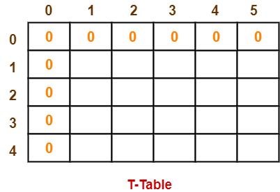
- Draw a table say ‘T’ with (n+1) = 4 + 1 = 5 number of rows and (w+1) = 5 + 1 = 6 number of columns.
- Fill all the boxes of 0th row and 0th column with 0.

Step-02:
Start filling the table row wise top to bottom from left to right using the formula-
T (i , j) = max { T ( i-1 , j ) , valuei + T( i-1 , j – weighti ) }
Finding T(1,1)-
We have,
- i = 1
- j = 1
- (value)i = (value)1 = 3
- (weight)i = (weight)1 = 2
Substituting the values, we get-
T(1,1) = max { T(1-1 , 1) , 3 + T(1-1 , 1-2) }
T(1,1) = max { T(0,1) , 3 + T(0,-1) }
T(1,1) = T(0,1) { Ignore T(0,-1) }
T(1,1) = 0
Finding T(1,2)-
We have,
- i = 1
- j = 2
- (value)i = (value)1 = 3
- (weight)i = (weight)1 = 2
Substituting the values, we get-
T(1,2) = max { T(1-1 , 2) , 3 + T(1-1 , 2-2) }
T(1,2) = max { T(0,2) , 3 + T(0,0) }
T(1,2) = max {0 , 3+0}
T(1,2) = 3
Finding T(1,3)-
We have,
- i = 1
- j = 3
- (value)i = (value)1 = 3
- (weight)i = (weight)1 = 2
Substituting the values, we get-
T(1,3) = max { T(1-1 , 3) , 3 + T(1-1 , 3-2) }
T(1,3) = max { T(0,3) , 3 + T(0,1) }
T(1,3) = max {0 , 3+0}
T(1,3) = 3
Finding T(1,4)-
We have,
- i = 1
- j = 4
- (value)i = (value)1 = 3
- (weight)i = (weight)1 = 2
Substituting the values, we get-
T(1,4) = max { T(1-1 , 4) , 3 + T(1-1 , 4-2) }
T(1,4) = max { T(0,4) , 3 + T(0,2) }
T(1,4) = max {0 , 3+0}
T(1,4) = 3
Finding T(1,5)-
We have,
- i = 1
- j = 5
- (value)i = (value)1 = 3
- (weight)i = (weight)1 = 2
Substituting the values, we get-
T(1,5) = max { T(1-1 , 5) , 3 + T(1-1 , 5-2) }
T(1,5) = max { T(0,5) , 3 + T(0,3) }
T(1,5) = max {0 , 3+0}
T(1,5) = 3
Finding T(2,1)-
We have,
- i = 2
- j = 1
- (value)i = (value)2 = 4
- (weight)i = (weight)2 = 3
Substituting the values, we get-
T(2,1) = max { T(2-1 , 1) , 4 + T(2-1 , 1-3) }
T(2,1) = max { T(1,1) , 4 + T(1,-2) }
T(2,1) = T(1,1) { Ignore T(1,-2) }
T(2,1) = 0
Finding T(2,2)-
We have,
- i = 2
- j = 2
- (value)i = (value)2 = 4
- (weight)i = (weight)2 = 3
Substituting the values, we get-
T(2,2) = max { T(2-1 , 2) , 4 + T(2-1 , 2-3) }
T(2,2) = max { T(1,2) , 4 + T(1,-1) }
T(2,2) = T(1,2) { Ignore T(1,-1) }
T(2,2) = 3
Finding T(2,3)-
We have,
- i = 2
- j = 3
- (value)i = (value)2 = 4
- (weight)i = (weight)2 = 3
Substituting the values, we get-
T(2,3) = max { T(2-1 , 3) , 4 + T(2-1 , 3-3) }
T(2,3) = max { T(1,3) , 4 + T(1,0) }
T(2,3) = max { 3 , 4+0 }
T(2,3) = 4
Finding T(2,4)-
We have,
- i = 2
- j = 4
- (value)i = (value)2 = 4
- (weight)i = (weight)2 = 3
Substituting the values, we get-
T(2,4) = max { T(2-1 , 4) , 4 + T(2-1 , 4-3) }
T(2,4) = max { T(1,4) , 4 + T(1,1) }
T(2,4) = max { 3 , 4+0 }
T(2,4) = 4
Finding T(2,5)-
We have,
- i = 2
- j = 5
- (value)i = (value)2 = 4
- (weight)i = (weight)2 = 3
Substituting the values, we get-
T(2,5) = max { T(2-1 , 5) , 4 + T(2-1 , 5-3) }
T(2,5) = max { T(1,5) , 4 + T(1,2) }
T(2,5) = max { 3 , 4+3 }
T(2,5) = 7
Similarly, compute all the entries.
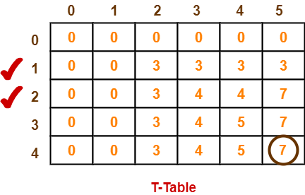
After all the entries are computed and filled in the table, we get the following table-

- The last entry represents the maximum possible value that can be put into the knapsack.
- So, maximum possible value that can be put into the knapsack = 7.
Identifying Items To Be Put Into Knapsack-
Following Step-04,
- We mark the rows labelled “1” and “2”.
- Thus, items that must be put into the knapsack to obtain the maximum value 7 are-
Item-1 and Item-2
To gain better understanding about 0/1 Knapsack Problem,
Next Article- Travelling Salesman Problem
Get more notes and other study material of Design and Analysis of Algorithms.
Watch video lectures by visiting our YouTube channel LearnVidFun.