Principal Component Analysis | Dimension Reduction

Dimension Reduction-

 

In pattern recognition, Dimension Reduction is defined as-

• It is a process of converting a data set having vast dimensions into a data set with lesser dimensions.
• It ensures that the converted data set conveys similar information concisely.

 

Example-

 

Consider the following example-

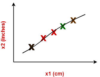
• The following graph shows two dimensions x1 and x2.
• x1 represents the measurement of several objects in cm.
• x2 represents the measurement of several objects in inches.

 

 

In machine learning,

• Using both these dimensions convey similar information.
• Also, they introduce a lot of noise in the system.
• So, it is better to use just one dimension.

 

Using dimension reduction techniques-

• We convert the dimensions of data from 2 dimensions (x1 and x2) to 1 dimension (z1).
• It makes the data relatively easier to explain.

 

 

Benefits-

 

Dimension reduction offers several benefits such as-

• It compresses the data and thus reduces the storage space requirements.
• It reduces the time required for computation since less dimensions require less computation.
• It eliminates the redundant features.
• It improves the model performance.

 

Dimension Reduction Techniques-

 

The two popular and well-known dimension reduction techniques are-

 

 

1. Principal Component Analysis (PCA)
2. Fisher Linear Discriminant Analysis (LDA)

 

In this article, we will discuss about Principal Component Analysis.

 

Principal Component Analysis-

 

• Principal Component Analysis is a well-known dimension reduction technique.
• It transforms the variables into a new set of variables called as principal components.
• These principal components are linear combination of original variables and are orthogonal.
• The first principal component accounts for most of the possible variation of original data.
• The second principal component does its best to capture the variance in the data.
• There can be only two principal components for a two-dimensional data set.

 

PCA Algorithm-

 

The steps involved in PCA Algorithm are as follows-

 

Step-01: Get data.

Step-02: Compute the mean vector (µ).

Step-03: Subtract mean from the given data.

Step-04: Calculate the covariance matrix.

Step-05: Calculate the eigen vectors and eigen values of the covariance matrix.

Step-06: Choosing components and forming a feature vector.

Step-07: Deriving the new data set.

 

PRACTICE PROBLEMS BASED ON PRINCIPAL COMPONENT ANALYSIS-

 

Problem-01:

 

Given data = { 2, 3, 4, 5, 6, 7 ; 1, 5, 3, 6, 7, 8 }.

Compute the principal component using PCA Algorithm.

 

OR

 

Consider the two dimensional patterns (2, 1), (3, 5), (4, 3), (5, 6), (6, 7), (7, 8).

Compute the principal component using PCA Algorithm.

 

OR

 

Compute the principal component of following data-

CLASS 1

X = 2 , 3 , 4

Y = 1 , 5 , 3

CLASS 2

X = 5 , 6 , 7

Y = 6 , 7 , 8

 

Solution-

 

We use the above discussed PCA Algorithm-

 

Step-01:

 

Get data.

The given feature vectors are-

• x₁ = (2, 1)
• x₂ = (3, 5)
• x₃ = (4, 3)
• x₄ = (5, 6)
• x₅ = (6, 7)
• x₆ = (7, 8)

 

 

Step-02:

 

Calculate the mean vector (µ).

 

Mean vector (µ)

= ((2 + 3 + 4 + 5 + 6 + 7) / 6, (1 + 5 + 3 + 6 + 7 + 8) / 6)

= (4.5, 5)

 

Thus,

 

Step-03:

 

Subtract mean vector (µ) from the given feature vectors.

• x₁ – µ = (2 – 4.5, 1 – 5) = (-2.5, -4)
• x₂ – µ = (3 – 4.5, 5 – 5) = (-1.5, 0)
• x₃ – µ = (4 – 4.5, 3 – 5) = (-0.5, -2)
• x₄ – µ = (5 – 4.5, 6 – 5) = (0.5, 1)
• x₅ – µ = (6 – 4.5, 7 – 5) = (1.5, 2)
• x₆ – µ = (7 – 4.5, 8 – 5) = (2.5, 3)

 

Feature vectors (x_i) after subtracting mean vector (µ) are-

 

 

Step-04:

 

Calculate the covariance matrix.

Covariance matrix is given by-

 

 

Now,

 

 

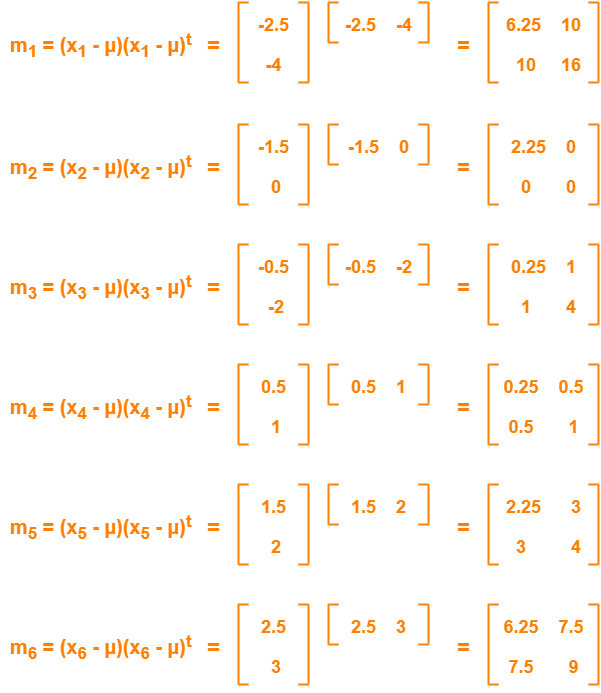
Now,

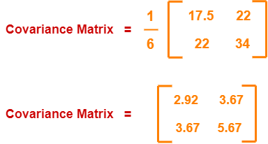
Covariance matrix

= (m₁ + m₂ + m₃ + m₄ + m₅ + m₆) / 6

 

On adding the above matrices and dividing by 6, we get-

 

 

Step-05:

 

Calculate the eigen values and eigen vectors of the covariance matrix.

λ is an eigen value for a matrix M if it is a solution of the characteristic equation |M – λI| = 0.

So, we have-

 

 

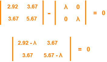
From here,

(2.92 – λ)(5.67 – λ) – (3.67 x 3.67) = 0

16.56 – 2.92λ – 5.67λ + λ² – 13.47 = 0

λ² – 8.59λ + 3.09 = 0

 

Solving this quadratic equation, we get λ = 8.22, 0.38

Thus, two eigen values are λ₁ = 8.22 and λ₂ = 0.38.

 

Clearly, the second eigen value is very small compared to the first eigen value.

So, the second eigen vector can be left out.

 

Eigen vector corresponding to the greatest eigen value is the principal component for the given data set.

So. we find the eigen vector corresponding to eigen value λ₁.

 

We use the following equation to find the eigen vector-

MX = λX

where-

• M = Covariance Matrix
• X = Eigen vector
• λ = Eigen value

 

Substituting the values in the above equation, we get-

 

 

Solving these, we get-

2.92X₁ + 3.67X₂ = 8.22X₁

3.67X₁ + 5.67X₂ = 8.22X₂

 

On simplification, we get-

5.3X₁ = 3.67X₂       ………(1)

3.67X₁ = 2.55X₂     ………(2)

 

From (1) and (2), X₁ = 0.69X₂

From (2), the eigen vector is-

 

 

Thus, principal component for the given data set is-

 

 

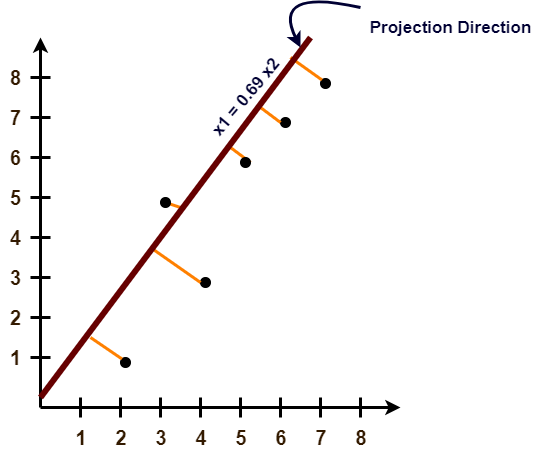
Lastly, we project the data points onto the new subspace as-

 

 

Problem-02:

 

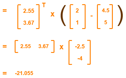
Use PCA Algorithm to transform the pattern (2, 1) onto the eigen vector in the previous question.

 

Solution-

 

The given feature vector is (2, 1).

 

The feature vector gets transformed to

= Transpose of Eigen vector x (Feature Vector – Mean Vector)

 

 

To gain better understanding about Principal Component Analysis,

Watch this Video Lecture

 

Get more notes and other study material of Pattern Recognition.

Watch video lectures by visiting our YouTube channel LearnVidFun.